Past exam of the general relativity and cosmology course of the University of Oxford / 2017 (A13484W1, B5)

Source paper: www-thphys.physics.ox.ac.uk/people/AndreiStarinets/TUTORIALS_NOTES_GR/gr_cosmology_exam_paper_2017.pdf

The lettered subdivisions index the successive separately marked blocks of each source question.

The covariant derivative differentiates a vector field while accounting for how its coordinate basis changes between neighboring points. For the Levi-Civita connection,The Christoffel symbol term makes this a tensor with one contravariant and one covariant index; ordinary partial derivatives of vector components do not generally have that transformation law. Equivalently, one compares the neighboring vector with the original after parallel transport.

For a curve $x^{\gamma }(\lambda )$ with tangent $U^{\gamma }=d{x}^{\gamma }/d\lambda$, contraction gives the covariant derivative along a curveIt is the rate of change measured relative to a parallel transport frame along the curve. It vanishes precisely when $v$ undergoes parallel transport along that curve. If $v=U$, it is the covariant acceleration, and its vanishing is the geodesic equation with an affine parameter.

Use metric signature $(-,+,+,+)$ and a bulk four-velocity normalized by $u^{\alpha }{u}_{\alpha }=-c^2$. A perfect fluid in general relativity is isotropic in its local rest frame, with no rest-frame energy flux or anisotropic stress. In an orthonormal frame in spacetime comoving with that fluid,Here $\rho$ is rest-frame energy density divided by $c^2$, including random kinetic energy, and $p$ is isotropic pressure. For a particle gas, $p=\frac{1}{3}\int \mathbf{p}\cdot \mathbf{v}dn$ and $\rho c^2=\int Edn$, with $dn$ the rest-frame particle distribution. Isotropy makes the off-diagonal spatial stresses and net energy flux vanish.

Introduce the spatial projector of a timelike congruenceThe only isotropic decomposition with the preceding components isSince both sides are tensors, equality in the comoving orthonormal frame in spacetime establishesCoordinate-independent definitions of the two scalar fields areThus $\rho$ is not, in general, only the sum of the particle rest masses per volume.

The microscopic averaging notation needs a normalization qualification. The normalization of an averaged four-velocity matters because a literal average of normalized microscopic four-velocities is not normally a normalized bulk four-velocity. For example, six equally weighted streams with the same ordinary speed $v$, directed along the positive and negative coordinate axes, have an isotropic velocity distribution andThe physical rest-frame bulk four-velocity is $(c,0,0,0)$, not this unnormalized average. Even taking the source's schematic kinetic expression literally with prefactor ${\rho }_s$ givesSubstituting $u=⟨v⟩$ and the same ${\rho }_s$ into the claimed fluid expression would instead increase $T^{00}$ by $p({\gamma }^2-1)$. The standard result therefore requires a normalized bulk velocity and a carefully defined rest-frame total energy density; it does not follow with both microscopic identifications interpreted literally. More generally the bulk velocity can be defined as the future-directed timelike energy eigenvector of the stress-energy tensor.

The equation ${\nabla }_{\alpha }{T}^{\alpha \beta }=0$ is local stress-energy conservation. In a weak gravitational field and the nonrelativistic limit its leading energy component gives mass conservation,while its spatial components give momentum conservation, or the inviscid Euler equationsThe next energy order gives conservation of internal plus kinetic energy, including pressure work and gravitational work. These are local conservation laws, not an assertion that arbitrary curved spacetimes possess a global conserved total energy.

For relativistic dust, $T^{\alpha \beta }=\rho u^{\alpha }{u}^{\beta }$, with $u^{\alpha }{u}_{\alpha }=-c^2$. Expanding stress-energy conservation givesContract with $u_{\beta }$. Metric compatibility and the fixed normalization implyConsequentlyThis is the covariant mass conservation equation. Substituting it back, wherever $\rho >0$, givesThus the dust's fluid elements follow timelike geodesics. With $u^{\alpha }=d{x}^{\alpha }/d\tau$, the proper time $\tau$ is an affine parameter, and explicitlyThe absence of pressure removes the force produced by pressure gradients; gravity is encoded by the Levi-Civita connection. At a point with $\rho =0$ this calculation makes no claim about a fluid velocity.

For nonrelativistic particles the energy density is dominated by rest energy, while their isotropic kinetic pressure is approximately $p_m=nm⟨v^2⟩/3$. ThereforeThe matter pressure is negligible in this approximation, including in the gravitational combination ${\rho }_m+3p_m/c^2$. For isotropic radiation in cosmology, $E=pc$ implies one third of the energy density in each diagonal spatial stress:

Because the two fluids do not exchange energy or momentum, they are separately conserved cosmological fluids: ${\nabla }_{\alpha }{T}_i^{\alpha \beta }=0$ for each, rather than merely conservation of their sum. In a comoving volume proportional to $a^3$, the first law of thermodynamics givesEquivalently this follows by projecting the individual stress-energy conservation equation along the common comoving four-velocity. Differentiating and dividing by ${\rho }_i{c}^2{a}^3$ yieldsFor constant equation-of-state parameter $w_i$,The extra power for radiation in cosmology represents the cosmological redshift of photon energies in addition to number dilution. Differentiating the total Friedmann equation gives only the total continuity equation; the separate equations also use the stated absence of interactions between components.

Both positive-density components have nonnegative pressure, so the Friedmann acceleration equation gives $\ddot{a}<0$ whenever $a>0$. Suppose $a(t_1)=a_1>0$ and $\dot{a}(t_1)=v_1>0$. Going backward while the solution is regular, $\dot{a}(t)\ge v_1$. Integrating,and thereforeA positive scale factor cannot persist indefinitely into the past: the right side vanishes at the finite time $t_1-a_1/v_1$.

For completeness, in this model the past endpoint must actually have $a\to 0$, rather than another singularity at positive $a$. From part (d) write ${\rho }_m=C_m/a^3$ and ${\rho }_r=C_r/a^4$ with $C_m,C_r>0$. ThenThe right side strictly decreases with $a$ and is positive at $a_1$, so it remains positive throughout $0<a<a_1$. There is no earlier bounce. It is smooth at every positive $a$, permitting continuation there. The lookback integral isNear $a=0$ its integrand is $a/\sqrt{K_r}$, which is integrable. ThusThe early asymptotic behavior is $a\simeq [2\sqrt{K_r}(t-t_0){]}^{1/2}$. Both densities diverge at this Big Bang boundary. Writing $a(t_0)=0$ denotes the limiting singular endpoint of the classical solution, not an ordinary regular spacetime slice.

Set $m=GM/c^2$ and $f(r)=1-2m/r$. A photon follows a null geodesic, with an affine parameter $\lambda$ satisfyingThe Christoffel symbols follow from the supplied Schwarzschild spacetime metric tensor. An efficient equivalent procedure is to use the geodesic Lagrangianwhere dots denote $d/d\lambda$. Its Euler-Lagrange equations give the affinely parametrized geodesic equations. The condition $\mathcal{L}=0$ is imposed after variation; setting the Lagrangian identically to zero before varying would discard the equations.

By spherical symmetry the ray's angular momentum fixes an orbital plane through the center. Rotate the angular coordinates so that plane is $\theta =\pi /2$. The $\theta$ Euler-Lagrange equation isso $\theta =\pi /2$, $\dot{\theta }=0$ is preserved once imposed initially. A radial ray has no unique orbital plane, but any plane through that radial line can be chosen.

The coordinates $t$ and $\varphi$ are cyclic. Thus their canonical momenta obeyThe two conserved quantities can be chosen asThese are the geodesic conserved quantities from Killing vectors ${\partial }_t$ and ${\partial }_{\varphi }$. With the chosen parameter normalization the conserved energy is $E=c^2\epsilon$ and axial angular momentum is $\ell$; multiplying the affine tangent by a constant multiplies both quantities by that constant.

The additional invariant is the squared norm of the affine tangent. Metric compatibility and the geodesic equation make it constant, and a photon has the null conditionOn the equatorial plane this givesand the conserved quantities of part (a) yieldFor a nonradial ray $\ell \ne 0$, put $u=1/r$. Sincethe orbit equation becomesHere $b=|\ell |/(c\epsilon )$ is the positive impact parameter for a future-directed ray arriving from infinity. A strictly radial ray has $\ell =0$ and must be described by the radial equation rather than by $\varphi$ as parameter.

The observer is static at $r_0$, with four-velocity $U=f_0^{-1/2}{\partial }_t$, where $f_0=1-2m/r_0$. Angles are measured in the observer's rest frame, using the positive spatial metric tensoron the equatorial plane. One cannot directly normalize a photon tangent with the full Lorentzian metric to define an angle, because that tangent is null.

At the observer the spatial direction of an outward-moving grazing ray is proportional to $w=A{\partial }_r+{\partial }_{\varphi }$, with $A=(dr/d\varphi {)}_{r_0}$. Its angle $\psi =\alpha /2$ to the outward radial direction equals the corresponding sky angle to the inward center of the image. Taking the spatial inner product with $e_r={\partial }_r$,ConsequentlyThe limiting value $A=0$ is understood by continuity.

For a grazing ray the areal radius has a turning point at the stellar surface $R$, so $\dot{r}=0$ there. The radial equation givesSince $R=4m>3m$, the surface lies outside the photon sphere. The function $f/r^2$ decreases for $r>3m$, so this tangential ray can escape to every $r_0>R$ and correctly defines the image's rim. For the specified surface,Also $dr/d\varphi =-r^{2}du/d\varphi$, henceIts sign depends on the orientation of the ray and of $\varphi$, and does not affect the angular diameter. Substitution givesThis apparent angular radius of a spherical star in Schwarzschild spacetime has useful limiting checks. As $r_0\downarrow R$, the star occupies a hemisphere, $\alpha \to \pi$. Far away, $\alpha \simeq 2b/r_0=8\sqrt{2}m/r_0$: Schwarzschild light deflection increases the apparent radius by a factor $\sqrt{2}$ relative to the flat-space value $R/r_0$.

Work consistently to first order in the metric perturbation, with ${\partial }_{\mu }{\xi }^{\nu }$ of the same small order. Under the passive change $x^{\prime \mu }=x^{\mu }+{\xi }^{\mu }(x)$,Applying this to the full metric tensor and writing $g_{\mu \nu }^{\prime }={\eta }_{\mu \nu }+h_{\mu \nu }^{\prime }$ with the same fixed numerical Minkowski metric givesIndices on $\xi$ are lowered with $\eta$. This is the gauge transformation of the perturbation relative to a fixed background. If the background were transformed as a tensor as well, the difference of those two fully transformed metrics would instead obey the homogeneous tensor transformation law. The inhomogeneous terms arise from retaining the fixed-background identification used in linearized gravity.

The trace changes by $h^{\prime }=h-2{\partial }_{\alpha }{\xi }^{\alpha }$, so the trace-reversed metric perturbation changes asLet $F_{\nu }={\partial }^{\mu }{\bar{h}}_{\mu \nu }$. Commuting partial derivatives givesThus choose a solution of the inhomogeneous wave equationSuch a solution exists locally with suitable initial data, and can be selected with appropriate wave-equation boundary conditions. This imposes the Lorenz gauge in linearized gravity, ${\partial }^{\mu }{\bar{h}}_{\mu \nu }^{\prime }=0$. All the divergence terms in the supplied vacuum equation then vanish, leavingThe remaining freedom $\square {\xi }_{\nu }=0$ is the residual gauge symmetry of linearized gravity.

Using the old coordinates in these derivatives is consistent at the retained order. IndeedActing on a first-order perturbation, the correction is a product of two first-order quantities and is discarded. Similarly replacing the argument $x^{\prime }$ by $x$ changes $h^{\prime }$ by $O(h^2)$ under the same perturbative ordering. This does not assert an exact equality of the two coordinate differential operators; it is the linear approximation about the fixed flat background.

For a nonzero plane-wave trace-reversed metric perturbation,The wave equation therefore requires a null wave vector. The Lorenz gauge in linearized gravity supplies transversality:The amplitude is symmetric because it represents a metric perturbation; its real part is the physical wave. The two displayed conditions do not by themselves make it spatially transverse and traceless: the additional reduction to transverse-traceless gauge uses the remaining residual gauge symmetry of linearized gravity.

Take the real physical wave and write $h(t,z)=A\cos [k(z-ct)]$. The specified amplitude has zero trace, so its metric perturbation equals its trace-reversed metric perturbation. It is in transverse-traceless gauge:to first order. Assume the freely falling particles are initially at rest in these coordinates. Since $g_{00}=-1$ and $g_{0i}=0$ in coordinates $(ct,x,y,z)$,The geodesic equations therefore admitUniqueness preserves these initial conditions. Thus the coordinate locations remain fixed; this conclusion does not apply to arbitrary initially moving particles.

Coordinate position is not measured separation. In the central observer's local orthonormal frame in spacetime, and in the long-wavelength limit appropriate to a small detector, the transverse physical separations areto first order. In particular the two principal semiaxes of the ring areFor a point at angular position $\phi$ the radial displacement isThe freely falling ring in transverse-traceless gauge alternates between ellipses elongated in the $x$ and $y$ directions. Its area is unchanged to first order. This is the plus gravitational wave polarization; the axes exchange their roles after half a period.

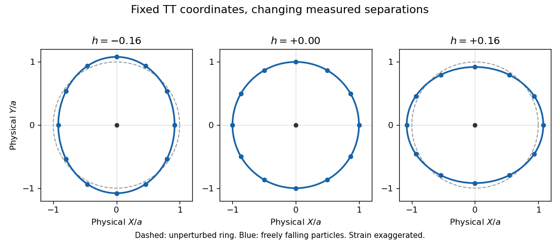
An observer at the center detects these changing distances, for example by exchanging light signals with the particles. Equivalently geodesic deviation gives the local tidal accelerationto the same order. There is physical relative motion and nonzero Riemann curvature tensor, even though the selected coordinate positions are constant. For a detector comparable to a wavelength, its light-travel-time response must be included rather than treating all distances as simultaneously measured local lengths.

Using the source's rounded solar mass, each hole has $m\simeq 3\times 10^{31}\mathrm{kg}$. Its Schwarzschild radius isThus $\boxed{r_s\sim 10^5\mathrm{m}}$ at order-of-magnitude accuracy. Using the more accurate solar mass would give about $9\times 10^4\mathrm{m}$.

The stated orbit is not a consistent separated-hole weak-field binary. Its nominal center-to-center separation is only $20\mathrm{km}$, below even the above single-hole radius. Applying two isolated Schwarzschild spacetime descriptions and a circular Newtonian orbit at that separation is not controlled. Likewise an estimate ${\bar{h}}_{11}^{\prime }\sim r_s/r$ at $r=10\mathrm{km}$ is of order one or larger, contradicting the small-perturbation assumption. The intended near-source statement is therefore a strong-field scale,not a reliable prediction from linearized gravity at the specified orbit. The exact radiative component is also gauge dependent near the source.

One can still estimate the intended distant gravitational wave strain scale. A radiative amplitude decreases as $1/D$ in the wave zone. A compact strong-field source has a characteristic length of order $r_s$, giving a dimensional strain estimate $h_{\mathrm{far}}\sim r_s/D$, up to mass, orientation and efficiency factors of order unity. This is also the strong-field dimensional scale suggested by far-zone quadrupole strain; it is not an application of the slow-motion formula to the inconsistent orbit.

With the supplied conversion,For a ring radius $a=4\times 10^3\mathrm{m}$, part (c) gives a single principal semiaxis displacement amplitudeThe difference of the two principal semiaxes has twice this amplitude. This is a conditional dimensional estimate of a physically plausible merger signal at that distance; the supplied close circular orbit does not define a self-consistent waveform or a precise amplitude.

Normalize the present scale factor to $a_0=1$. Conservation of the number of electrons associated with the baryons makes their physical number density scale as $a^{-3}$. At this early epoch they are free rather than bound in neutral atoms, soHere the specified present density is interpreted as the conserved total electron abundance, including electrons that might be bound today. A present free-electron density would require an ionization-fraction correction.

Density alone does not determine whether a gas is relativistic; its random kinetic energy must be compared with the rest energy. In the usual thermal Hot Big Bang model, use the measured cosmic microwave background temperature $T_0\simeq 2.7\mathrm{K}$ and the temperature scaling of thermal photon number and energy densities, $T_{\gamma }\propto a^{-1}$. Tight coupling then givesSince $m_e{c}^2\simeq 5.1\times 10^5\mathrm{eV}$,Their thermal speed is of order $\sqrt{3k_B{T}_e/m_e}\simeq 0.04c$. The gas is fully ionized because its temperature is far above the recombination temperature, but ionization does not imply relativistic electrons. Thermal electron-positron pairs are exponentially suppressed at this temperature.^[ref]

The given age and scale-factor ratio should be treated as independent supplied estimates in the following rate comparison. They do not describe the same epoch in standard radiation-era expansion: $a/a_0=10^{-6}$ normally corresponds to an age of order a year, not $10^4$ years. The density and temperature estimates above depend on the scale-factor ratio, not on assigning it the stated age.

For statistically independent Thomson scattering events, the probability of no scattering over a proper distance $s$ is $\exp (-n_e{\sigma }_{e}s)$. The photon mean free path in an ionized universe is thereforeThis is about half an astronomical unit. It is a proper distance at that epoch, not a present-day comoving distance. The Thomson scattering approximation is appropriate because the electrons are nonrelativistic and typical photon energies are much smaller than $m_e{c}^2$. The source's spelling of the process is a typographical error; the physical process is Thomson scattering.

A photon travels at $c$, so its typical scattering interval isabout four minutes. The supplied universe age isThusA photon scatters extremely frequently compared with the expansion timescale, of order the cosmic age. The plasma is opaque and its photons are tightly coupled to the electrons rather than freely streaming over a cosmological distance. In rate language ${\Gamma }_{\gamma }=n_e{\sigma }_{e}c\gg H$, where $H$ is the Hubble parameter.^[ref]

This is a statement about transport and momentum coupling. Elastic Thomson scattering alone does not create or destroy photons and hence is not, by itself, proof that an arbitrary photon spectrum reaches complete blackbody thermal equilibrium. The interaction interval calculated here is the interval experienced by a photon; the interval per electron differs because there are many more photons than electrons. Even replacing the inconsistent supplied age by the standard age of order a year at this scale factor would leave scattering much faster than expansion.

As the temperature falls, electrons and protons form neutral hydrogen through cosmological recombination. The free electron fraction drops sharply, and so does the scattering rate ${\Gamma }_{\gamma }=n_e{\sigma }_{T}c$. When this rate becomes comparable to or smaller than the Hubble parameter, the plasma becomes transparent and photon decoupling occurs. The Thomson scattering cross-section itself does not abruptly vanish. The rapid change is in the abundance of free targets.

The Hydrogen binding energy is $13.6\mathrm{eV}$, but recombination occurs at a much smaller thermal energy, of order $0.3\mathrm{eV}$, or a few thousand kelvin. There are roughly a billion photons per baryon, so the high-energy tail can keep hydrogen ionized long after $k_{B}T$ drops below the binding energy. The falling exponential ionizing tail then makes the transition comparatively sharp. Last scattering follows when sufficiently few electrons remain free.^[ref]

To estimate a horizon, specify an expansion model as well as the redshift. The proper particle horizon at emission isAs a transparent analytic estimate, approximate a spatially flat matter-dominated universe by $a(t)=(t/t_{\mathrm{now}}{)}^{2/3}$ throughout. ThenTaking the illustrative present value $H_0=70\mathrm{km}{\mathrm{s}}^{-1}\mathrm{Mp}{\mathrm{c}}^{-1}$, this model has $t_{\mathrm{now}}=2/(3H_0)\simeq 9.3\times 10^9\mathrm{yr}$. At $z_{\ast }=10^3$,This is a proper horizon radius at emission; its corresponding present comoving length is about $270\mathrm{Mpc}$.

For the same model the comoving distance to the Cosmic microwave background last-scattering surface and its angular diameter distance areTherefore the angular extent associated with one radial horizon length isThis is an order-one-degree estimate. Including the earlier radiation domination and late dark energy changes the coefficient; it does not make the horizon span the sky. A horizon patch diameter has twice this angle, whereas the acoustic scale uses a sound horizon and differs again. The redshift by itself, without an expansion model or normalization, is insufficient for a unique horizon distance.

The horizon problem is that the observed cosmic microwave background has nearly the same mean temperature across angular separations vastly greater than this scale. In the purely decelerating Hot Big Bang model, sufficiently separated last-scattering regions had neither time to exchange signals nor a common post-Big-Bang causal region that could establish their observed thermal uniformity. The puzzle concerns the missing causal explanation of those initial correlations; it is not an inconsistency of specifying uniform initial conditions mathematically. An earlier period of cosmic inflation can enlarge a formerly causally connected region beyond the later observable horizon.