General relativity and cosmology course of the University of Oxford (B5, B3)

Solution

In general coordinates the basis changes along the world line. Differentiating only the components of a vector omits that basis change, and does not transform as a vector under a position-dependent coordinate transformation. The appropriate rate is the covariant derivative along a curve:

\frac{D V ^{α}}{d λ} = \frac{d V ^{α}}{d λ} + Γ^{α}_{β γ} \frac{d x ^{β}}{d λ} V^{γ} .

For the metric-compatible torsion-free connection, the Christoffel symbols are determined by the metric tensor and its first derivatives:

Γ^{α}_{β γ} = \frac{1}{2} g^{α δ} (\partial_{β} g_{δ γ} + \partial_{γ} g_{δ β} - \partial_{δ} g_{β γ}) .

Thus the ship's four-acceleration is

a^{α} = \frac{D u ^{α}}{d τ} = \frac{d u ^{α}}{d τ} + Γ^{α}_{β γ} u^{β} u^{γ} .

In Cartesian coordinates of an inertial frame in flat spacetime, the connection coefficients vanish and the ordinary component derivative happens to suffice. In curved spacetime it suffices at a chosen event in a local inertial frame, but not generally along an extended trajectory.

c

Solution

Use metric signature

(-, +, +, +)

and

x^{0} = c t

. At an event in the ship's instantaneous rest local inertial frame,

u^{α} = (c, 0, 0, 0)

. Since its squared norm is a scalar,

u^{α} u_{α} = - c^{2}

in every coordinate system. Equivalently it follows directly from

d s^{2} = - c^{2} d τ^{2}

and

u^{α} = d x^{α} / d τ

Metric compatibility lets us differentiate this identity covariantly:

0 = \frac{D}{d τ} (g_{α β} u^{α} u^{β}) = 2 u_{α} a^{α}, u_{α} a^{α} = 0.

In the instantaneous rest local inertial frame, the last equation gives

a^{0} = 0

. The spatial components are the acceleration recorded by an onboard accelerometer,

a_{rest}

, whose magnitude is

g

. Therefore

a^{α} a_{α} = ∣ a_{rest} ∣^{2} = g^{2} .

This proper acceleration is zero in ideal free fall, even when the coordinate position has a nonzero second derivative. A coordinate acceleration and an accelerometer reading are different quantities.

d

Solution

Put

F (r) = 1 - r_{s} / r

and

r_{s} = 2 GM / c^{2}

. For radial motion

u^{θ} = u^{ϕ} = 0

. The given Christoffel symbols imply

a^{0} = \frac{d u ^{0}}{d τ} + \frac{2 GM}{c ^{2} r ^{2} F} u^{0} u^{r},

and

a^{r} = \frac{d u ^{r}}{d τ} + \frac{GM}{c ^{2} r ^{2}} [F (u^{0})^{2} - F^{- 1} (u^{r})^{2}] .

The four-velocity normalization of part c is

- F (u^{0})^{2} + F^{- 1} (u^{r})^{2} = - c^{2} .

Its bracketed combination is therefore exactly

c^{2}

, independently of the instantaneous velocity or the thrust history. Consequently

a^{r} = \frac{d u ^{r}}{d τ} + \frac{GM}{r ^{2}} .

The derivative here is with respect to proper time. This expression does not say that the ship measures a gravitational acceleration

GM / r^{2}

during free fall; setting

a^{r} = 0

gives its radial proper-time equation of motion in Schwarzschild spacetime.

e

Solution

For radial motion outside the Schwarzschild event horizon, the equations needed to determine the acceleration components are

- F (u^{0})^{2} + F^{- 1} (u^{r})^{2} - F u^{0} a^{0} + F^{- 1} u^{r} a^{r} - F (a^{0})^{2} + F^{- 1} (a^{r})^{2} = - c^{2}, = 0, = g^{2} .

They are respectively the four-velocity norm, velocity-acceleration orthogonality, and the maximum proper acceleration norm. Together with part d they give the stated thrust equation; no integration of the trajectory is required. The positive radial sign corresponds to outward thrust.

Let

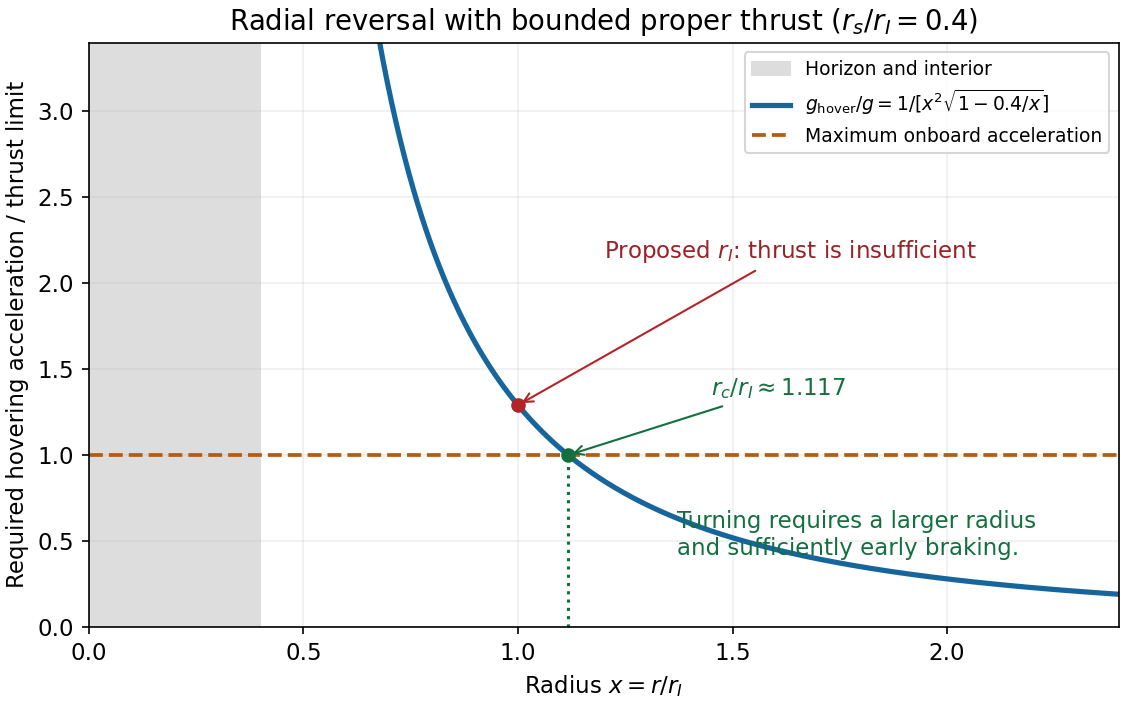
r_{I} = GM / g

. A first transition from inward to outward motion requires

u^{r} = 0

at a minimum radius and

d u^{r} / d τ \geq 0

there. The largest possible radial derivative at such an event is

\frac{d u ^{r}}{d τ}_{u^{r} = 0} = g 1 - r_{s} / r - \frac{GM}{r ^{2}} .

r = r_{I} > r_{s}

, this is

\frac{d u ^{r}}{d τ}_{r_{I}, u^{r} = 0} = g [1 - r_{s} / r_{I} - 1] < 0.

Thus the ship cannot reverse its inward motion there. It cannot reverse at any smaller exterior radius either:

GM / r^{2}

grows while

1 - r_{s} / r

decreases. If it first reaches

r_{I}

while falling inward, it cannot return home using the stipulated bounded radial thrust. If

r_{I} \leq r_{s}

, it would instead have reached the black-hole horizon before that radius, which already prevents escape.

The minimum radius for radial turnaround with bounded proper acceleration lies strictly outside the proposed radius. Define

r_{c} > r_{s}

g = \frac{GM}{r _{c}^{2} 1 - r _{s} / r _{c}} .

The right side is the proper acceleration required to hover, decreases monotonically from infinity to zero, and exceeds

GM / r^{2}

. A genuine turnaround needs

r_{turn} > r_{c} > r_{I}

; equality gives no positive initial outward acceleration at rest. A sufficiently early burn is also needed to remove the pre-existing inward velocity. The failure at

r_{I}

follows from the turning-point condition, not from treating the moving ship as static throughout its fall.

Figure 1.
The Newtonian proposed radius lies inside the bounded-thrust turnaround limit
. For the illustrative ratio rs/rI equal to 0.4, the curve is the required hovering proper acceleration divided by the maximum onboard acceleration. At rI it exceeds one. Its crossing with one determines the critical radius rc; the outer side is necessary for radial reversal. The black-hole interior is excluded from this static-coordinate comparison. **Details**.

2

a

Solution

In coordinates

(c t, r, ϕ, z)

the diagonal metric tensor is

diag (- 1, 1, f^{2}, 1)

, and only

g_{ϕϕ}

depends on position. Substitution into the connection formula gives

Γ^{r}_{ϕϕ} = - f f^{'}, Γ^{ϕ}_{r ϕ} = Γ^{ϕ}_{ϕ r} = \frac{f ^{'}}{f},

with all other Christoffel symbols zero away from singular axes.

Use the explicit Ricci tensor formula and the Einstein equation sign printed on the source formula sheet. They give

R_{rr} = \frac{f ^{''}}{f}, R_{ϕϕ} = f f^{''}, R = g^{α β} R_{α β} = 2 \frac{f ^{''}}{f} .

For example, in

R_{rr}

the two terms proportional to

(f^{'} / f)^{2}

cancel. For

R_{ϕϕ}

the derivative of

- f f^{'}

contributes

(f^{'})^{2} + f f^{''}

, the product terms contribute

- 2 (f^{'})^{2}

, and the determinant term contributes

(f^{'})^{2}

Formula-sheet qualification. Directly contracting the separately printed Riemann curvature tensor as instructed on that sheet instead gives

R_{rr} = - f^{''} / f

, the opposite sign. For the concrete example

f (r) = ℓ sin (r / ℓ)

, that contraction gives

+ 1/ ℓ^{2}

, whereas the explicit Ricci tensor formula gives

- 1/ ℓ^{2}

. The two source formulas cannot both hold with the stated contraction. The calculation here uses the explicit Ricci tensor formula, whose pairing with the negative Einstein equation coupling yields the requested stress-energy tensor.

The desired matter tensor assumes

Λ = 0

; otherwise the cosmological-constant contribution must also be included. With that assumption,

T_{α β} = - \frac{c ^{4}}{8 π G} (R_{α β} - \frac{1}{2} g_{α β} R),

and raising both indices gives

T^{α β} = \frac{c ^{4}}{8 π G} \frac{f ^{''}}{f} diag (- 1, 0, 0, 1) .

The static observer measures energy density

T^{00} = - c^{4} f^{''} / (8 π G f)

and equal-magnitude negative axial pressure when that energy is positive. The axial stress is a tension. Keeping the source's curvature sign and its negative Einstein-equation coupling together is essential to this result.

b

Solution

Assume

ϕ

has period

2 π

f > 0

in the regular bulk, and consider a unit proper length in

z

. The proper transverse area element is

d A = f d r d ϕ

, while the mass density is

T^{00} / c^{2}

. The axial boundary term in the mass of a cylindrical spacetime is therefore

μ_{bulk} = \int_{0}^{R} \frac{T ^{00}}{c ^{2}} 2 π f d r = - \frac{c ^{2}}{4 G} \int_{0}^{R} f^{''} d r = \frac{c ^{2}}{4 G} [f^{'} (0^{+}) - f^{'} (R^{-})] .

Choose the usual deficit branch

0 \leq λ < 1

, so

f_{out} = (1 - λ) r

. Continuity of the induced metric requires

f (R^{-}) = (1 - λ) R

. If there is no distributional thin shell at

R

, continuity of the extrinsic curvature also requires

f^{'} (R^{-}) = 1 - λ

. A jump in

f^{'}

would add a surface-layer stress and cannot simply be discarded.

Using the printed inner condition

f^{'} (0^{+}) = 0

, these assumptions yield

μ_{bulk} = \frac{c ^{2}}{4 G} (λ - 1) .

This is the literal smooth-bulk answer. It is negative for the ordinary deficit range, so it must not be silently replaced by the usual positive cosmic-string mass formula.

For comparison, a regular axis with proper radial coordinate and angular period

2 π

requires

f (0) = 0

and

f^{'} (0) = 1

, since the circumference-to-radius ratio must approach

2 π

. Under that different regular-axis condition the same integral gives

μ_{regular} = \frac{λ c ^{2}}{4 G}, δ = 2 πλ = \frac{8 π G μ _{regular}}{c ^{2}} .

The original PDF really prints the derivative limit zero. It describes either a nonregular axis or an inner geometry different from an ordinary smooth string core; any additional singular-axis matter is not included in the bulk integral above and would need its own stress specification. Standard regular-core matching can also require an offset in the exterior radial origin. Thus the regular-axis formula is a qualified physical interpretation, not a derivation from the printed zero. For a general exterior branch replace

1 - λ

∣1 - λ ∣

in the boundary derivative.

c

Solution

Outside the core,

f^{''} = 0

and the metric is locally flat: set

ϕ = (1 - λ) ϕ

. Static test particles have no Newtonian-like attraction because

g_{00}

is constant and

Γ^{r}_{00} = 0

. Local trajectories are straight lines in locally unwrapped coordinates, so a very thin dark core is hard to identify through ordinary orbital accelerations or local tidal forces.

The global angular range is nevertheless

2 π (1 - λ)

rather than

2 π

. The missing angle

δ = 2 πλ

can give gravitational lensing with two nearly identical, essentially undistorted images of a background galaxy, and multiple such pairs aligned along the projected object. For a small deficit, a straight string and favourable geometry, their angular separation is of order

δ D_{l s} / D_{s}

, with an additional inclination factor for a tilted string. The matching spectra and common line of image pairs distinguish this from an ordinary compact lens.

A moving cosmic string can also induce a step in the cosmic microwave background temperature across its path. That signature needs motion in addition to the static geometry supplied here. These are consequences of the exterior conical geometry; interpreting the inferred deficit as a positive mass per length requires the regular-axis/core assumptions distinguished in part b.

3

a

Solution

The cosmic distance ladder starts by calibrating a physical baseline. Radar echoes from planets or spacecraft give a round-trip light time and hence a distance

d = c Δ t /2

, after accounting for orbital motion and propagation delays. Combining this with orbital geometry fixes the Earth-Sun orbital scale; directly timing a reflected pulse from the solar surface is not required.

That baseline supplies annual stellar parallax: for small parallax angle

p

d ≃ b / p

, or

d

in parsecs equals

1/ p

when

p

is in arcseconds and

b

is one astronomical unit. Nearby parallax distances calibrate stellar absolute magnitudes. Main-sequence fitting extends the scale to star clusters, and the calibrated Cepheid period-luminosity relation gives luminosities for Cepheids visible in nearby galaxies.

Cepheid-host galaxies then calibrate Type Ia supernovae. After light-curve and colour standardization, their high luminosities permit distances to much more remote galaxies. For a source of calibrated luminosity

L

and observed bolometric flux

F

d_{L} = \frac{L}{4 π F}, m - M = 5 lo g_{10} (\frac{d _{L}}{10 pc})

with consistent bandpass definitions and corrections. Interstellar extinction, composition, stellar-population differences and calibration uncertainty must be propagated through the steps. Redshift can subsequently provide a distance within a fitted cosmological model; using it alone cannot independently calibrate the Hubble constant.

b

Solution

Normalize the scale factor to

a (t) = R (t) / R (t_{0})

, with

a (t_{0}) = 1

. Along a radial null geodesic,

d χ = c d t / a (t)

. Two successive wave crests sent by the same comoving emitter and received by the same comoving observer traverse the same comoving distance, so

\int_{t_{e}}^{t_{0}} \frac{c d t}{a ( t )} = \int_{t_{e} + δ t_{e}}^{t_{0} + δ t_{0}} \frac{c d t}{a ( t )} .

To first order,

δ t_{0} / a (t_{0}) = δ t_{e} / a (t_{e})

. Frequencies are inverse proper periods for the comoving observers, giving the cosmological redshift

1 + z = \frac{λ _{0}}{λ _{e}} = \frac{R ( t _{0} )}{R ( t _{e} )} = \frac{1}{a ( t _{e} )} .

Expansion stretches wavelengths, so a spectral line of known rest wavelength gives

z = λ_{obs} / λ_{rest} - 1

At small

z

, the light travel time is short compared with the expansion time. Expanding

R (t_{e})

gives

z ≃ H_{0} (t_{0} - t_{e})

and

d ≃ c (t_{0} - t_{e})

, hence

cz ≃ H_{0} d, H_{0} = \frac{R ˙}{R}_{t_{0}} .

Combine independently calibrated luminosity distances with galaxy spectral redshifts and fit the slope. Nearby peculiar velocities must be allowed for, while high-redshift data require the full distance-redshift relation rather than the linear approximation.

c

Solution

Use standardized Type Ia supernovae as distance indicators and measure their redshifts. The curvature of the luminosity-distance relation constrains the deceleration parameter:

d_{L} (z) = \frac{c}{H _{0}} [z + \frac{1 - q _{0}}{2} z^{2} + O (z^{3})], q_{0} = - \frac{R ¨ ( t _{0} )}{R ( t _{0} ) H _{0}^{2}} .

Fainter supernovae at a given redshift imply larger distances, and comparison with the predicted curve tests accelerated expansion. In practice one fits the full expansion history over the observed redshift range and controls luminosity evolution, extinction and calibration, rather than relying only on a short low-

z

series.

The cosmological fate from local expansion data is conditional on a matter model. For the spatially flat model of part b, if the only relevant components are pressureless matter and a constant

Λ

, put

A_{0} = \ddot{R} (t_{0}) / R (t_{0})

. The two Friedmann equations give

ρ_{m 0} = \frac{H _{0}^{2} - A _{0}}{4 π G}, Λ c^{2} = H_{0}^{2} + 2 A_{0} .

Here

Λ

follows the sign of the supplied Friedmann equations, where positive

Λ

contributes positive acceleration. These fix the parameters governing subsequent evolution. Positive

Λ

yields eternal late-time accelerated expansion; zero

Λ

gives the flat matter solution; negative

Λ

leads to eventual recollapse in this dust model. If instead one assumes dust and zero

Λ

while allowing curvature,

q_{0} = Ω_{m 0} /2

determines whether the matter universe is closed and recollapsing or expands indefinitely.

Without a fixed equation of state and its future evolution, two present derivatives do not uniquely fix the future. For a concrete counterexample in units with

t_{0} = 0

, the positive scale factors

a_{+} (t) = 1 + t + t^{2} /2

and

a_{-} (t) = 1 + t + t^{2} /2 - t^{3}

have the same

a, \overset{a}{˙}, \overset{a}{¨}

now. The former expands forever; the latter turns around and later reaches zero. Different time-dependent matter stresses can support their different flat expansion histories. Thus the printed sufficiency statement needs the cosmological-model assumption.

d

Solution

In an Einstein-de Sitter universe, take

a (t) = (t / t_{0})^{2/3}

and

t_{0} = 2/ (3 H_{0})

. The galaxy seen today at

z = 1

emitted the light now reaching us when

a (t_{e}) = 1/2

, so

t_{e} / t_{0} = 2^{- 3/2}

. Its fixed comoving radial distance is

χ = c \int_{t_{e}}^{t_{0}} \frac{d t}{a ( t )} = 3 c t_{0} (1 - \frac{1}{2}) .

Put

b = 1 - 1/ 2

. A new message sent now reaches the galaxy at

t_{1}

, where

χ = 3 c t_{0} [(t_{1} / t_{0})^{1/3} - 1], \frac{t _{1}}{t _{0}} = (1 + b)^{3} .

Assume an immediate reply and negligible local handling delays. The return consumes the same additional conformal time, giving the Einstein-de Sitter round-trip message time

\frac{t _{2}}{t _{0}} = (1 + 2 b)^{3} = (3 - 2)^{3} ≃ 3.98781, Δ t = t_{2} - t_{0} ≃ 2.98781 t_{0} = \frac{1.99187}{H _{0}} .

For the numerical value

H_{0} = 72 km s^{- 1} Mp c^{- 1}

supplied later in the paper,

H_{0}^{- 1} = 13.58 Gyr

and the waiting time is about

27.1 Gyr

. The age

t_{0} = 9.05 Gyr

here belongs to the stipulated matter-only model, not a claim about the actual measured cosmic age.

After

n

one-way legs,

t_{n} = t_{0} (1 + nb)^{3}

. Since

\int_{t_{0}}^{\infty} d t / a (t) = \infty

, every finite number of messages is possible and there is no finite fundamental upper count. The exchange takes arbitrarily long, with successively longer intervals; infinitely many messages are not completed in finite cosmic time.

Figure 1.
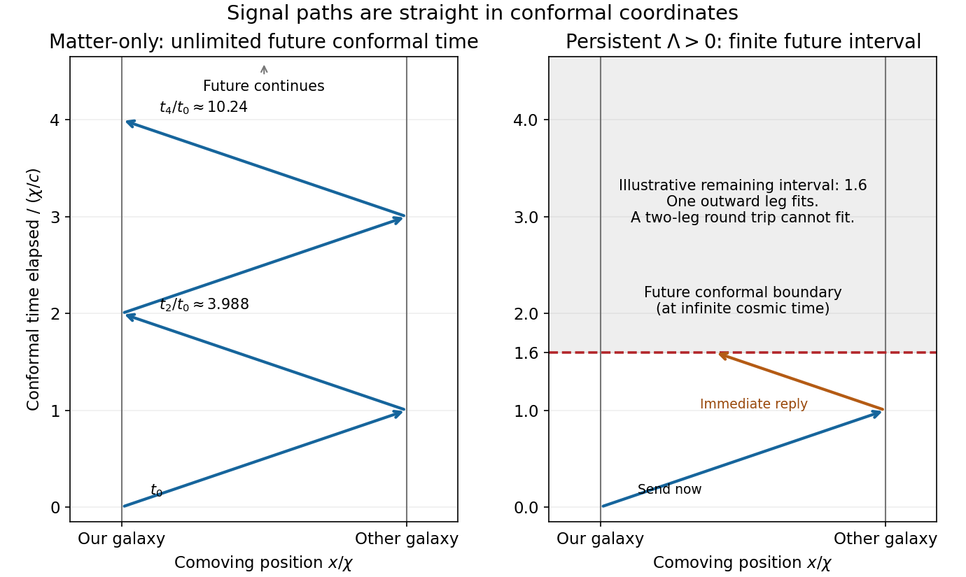
Message exchange depends on the remaining conformal time, not just the present expansion rate
. The left conformal spacetime diagram shows repeated light-signal legs between two comoving galaxies in an Einstein-de Sitter model. The right diagram illustrates a finite future conformal interval: one outward leg fits but a complete round trip does not. The right interval is a schematic example, not a parameter estimate for our Universe. **Details**.

e

Solution

Spatial flatness constrains the total density, not matter alone. A flat model can have

Ω_{m 0} + Ω_{Λ0} + Ω_{r 0} = 1

with a substantial dark energy component. A positive cosmological constant has pressure

p_{Λ} = - ρ_{Λ} c^{2}

and does not dilute like matter; it can produce the observed accelerated expansion.

If positive

Λ

persists,

a (t)

becomes exponential and the future conformal time interval

Δ η_{future} = \int_{t_{0}}^{\infty} \frac{d t}{a ( t )}

is finite. For two comoving civilisations separated by

χ

, each one-way signal consumes

χ / c

. Thus a message completing

n

legs at finite time requires

n \frac{χ}{c} < Δ η_{future} .

Only finitely many legs, and hence finitely many full exchanges, can then occur. A reply to even the first new message requires

2 χ / c < Δ η_{future}

, the cosmological round-trip communication horizon condition. Depending on the density parameters, the initial outward message might arrive while its reply can never reach us, as in the right-hand panel of part d.

The source gives no matter and dark-energy fractions, so it does not specify an exact count for the

z = 1

pair in the real Universe. Flatness and lack of matter dominance alone do not prove a finite horizon: a radiation-dominated flat universe, for example, has divergent future conformal time if that power-law expansion persists. The finite-message conclusion uses persistent accelerated expansion such as positive constant

Λ

4

a

Solution

For a photon gas in thermal and chemical equilibrium, photon number is not a conserved thermodynamic charge. Number-changing processes can create and absorb photons without a corresponding conserved-number constraint, so the equilibrium photon chemical potential is zero.

T = 5 \times 1 0^{9} K

k_{B} T ≃ 0.431 MeV

. The other light species are electrons, Positrons, three neutrino species and their antiparticles. Neutrinos are ultrarelativistic; electrons and Positrons are only moderately relativistic at this particular temperature because

m_{e} c^{2} = 0.511 MeV

. The later simple counting formulas use the intended ultrarelativistic approximation for them. Baryons, muons and heavier particles are not an abundant relativistic bath at this temperature.

Pair equilibrium implies

μ_{e^{-}} + μ_{e^{+}} = 2 μ_{γ} = 0

. Approximate charge symmetry, with the net electron excess tied to the much smaller baryon asymmetry, then makes both electron and Positron chemical potentials small compared with

k_{B} T

. For neutrinos one additionally assumes negligible lepton asymmetry. Their near-zero chemical potentials are not implied merely by their statistics. After neutrino decoupling, a distribution initially having negligible chemical potential retains a redshifted Fermi-Dirac distribution, with its own temperature.

b

Solution

Let

V

be proper volume, let

g_{i}

count the populated internal states, and take

μ_{i} = 0

and

ϵ = p c

. Spherical integration in momentum space gives

\frac{N _{i}}{V} = \frac{g _{i}}{2 π ^{2}} (\frac{k _{B} T}{ℏ c})^{3} \int_{0}^{\infty} \frac{x ^{2} d x}{e ^{x} \mp 1}, x = \frac{p c}{k _{B} T} .

Using the fermion-to-boson thermal integral ratio, the minus-denominator boson integral is

2 ζ (3)

and the plus-denominator fermion integral is

3 ζ (3) /2

. Hence

N_{B} = \frac{g _{B} ζ ( 3 )}{π ^{2}} V (\frac{k _{B} T}{ℏ c})^{3}, N_{F} = \frac{3}{4} \frac{g _{F} ζ ( 3 )}{π ^{2}} V (\frac{k _{B} T}{ℏ c})^{3} .

The energy integral has one extra factor

p c = k_{B} T x

\frac{U _{i}}{V} = \frac{g _{i}}{2 π ^{2}} \frac{( k _{B} T ) ^{4}}{( ℏ c ) ^{3}} \int_{0}^{\infty} \frac{x ^{3} d x}{e ^{x} \mp 1} .

The supplied distribution identity gives the fermion integral as

(1 - 2^{- 3}) π^{4} /15 = 7 π^{4} /120

. Therefore

U_{B} = \frac{g _{B} π ^{2}}{30} V \frac{( k _{B} T ) ^{4}}{( ℏ c ) ^{3}}, U_{F} = \frac{7}{8} \frac{g _{F} π ^{2}}{30} V \frac{( k _{B} T ) ^{4}}{( ℏ c ) ^{3}} .

For an isotropic ultrarelativistic gas, momentum flux gives

P_{i} = \frac{1}{3} \int p v f_{i} d^{3} p

. Since

v = c

and

p c = ϵ

P_{i} = \frac{U _{i}}{3 V} .

Photons have

g_{γ} = 2

, electrons and Positrons each have

g = 2

, and each neutrino or antineutrino species has one populated helicity in the standard thermal bath.

c

Solution

For zero chemical potential, each species contributes

S_{i} = (U_{i} + P_{i} V) / T = 4 U_{i} / (3 T)

. Thus

\frac{S _{B}}{V} = \frac{2 π ^{2}}{45} g_{B} k_{B} (\frac{k _{B} T}{ℏ c})^{3}, \frac{S _{F}}{V} = \frac{7}{8} \frac{2 π ^{2}}{45} g_{F} k_{B} (\frac{k _{B} T}{ℏ c})^{3} .

Entropy density scales as

T^{3}

at fixed relativistic particle content; total entropy also includes the changing proper volume. An isolated adiabatically expanding comoving gas has conserved total entropy and

a T

constant, rather than its total entropy falling as

T^{3}

At equal temperature, single electrons and photons each have two spin/polarization states. In the ultrarelativistic approximation,

\frac{S _{e^{-}}}{S _{γ}} = \frac{7}{8} .

Positrons are a separate species with the same contribution, so

(S_{e^{-}} + S_{e^{+}}) / S_{γ} = 7/4

. This distinction is needed for the heating count in part d. At the exact supplied temperature the electron rest mass gives corrections to the ideal

7/8

ratio; it is the limiting relativistic value requested by the problem.

There is also a sign convention issue in the introductory entropy formula. With the chemical-potential convention used in the supplied distribution, the Euler relation is

U = TS - P V + \sum_{i} μ_{i} N_{i}

, so

S = (U + P V - \sum_{i} μ_{i} N_{i}) / T

. Its chemical-potential term has the opposite sign to the printed one. For a concrete counterexample, a dilute monatomic ideal gas with one internal state and

n λ_{T}^{3} = e^{- 1}

, where

λ_{T}

is the thermal de Broglie wavelength, has

μ = - k_{B} T

U = 3 N k_{B} T /2

and

P V = N k_{B} T

. Its entropy is

7 N k_{B} /2

; the printed plus sign would instead give

3 N k_{B} /2

. All chemical potentials have been neglected here, so this source error does not change any of the above results.

d

Solution

As the plasma cools through electron-positron annihilation, the pairs transfer their entropy to the coupled photons. Neutrinos have largely decoupled and do not share that heating in the instantaneous-decoupling approximation. Before annihilation the electromagnetic entropy count is

g_{* s, before} = 2 + \frac{7}{8} (2 + 2) = \frac{11}{2},

while after it

g_{* s, after} = 2

. Conservation of electromagnetic comoving entropy,

g_{* s} T_{γ}^{3} a^{3} = constant

, gives the relative photon heating factor

\frac{( a T _{γ} ) _{after}}{( a T _{γ} ) _{before}} = (\frac{11}{4})^{1/3} ≃ 1.401.

Equivalently

T_{γ} / T_{ν} = (11/4)^{1/3}

afterward. The exact

11/4

count compares an asymptotic relativistic pair bath with the pair-free bath; at the supplied temperature some finite-electron-mass entropy loss has already begun.

The word “rises” requires care. The photons become hotter than an otherwise freely redshifting bath at the same scale factor; their absolute temperature need not rise during the expansion. In the smooth equilibrium process,

\frac{d ln T _{γ}}{d ln a} = - \frac{3}{3 + d ln g _{* s} / d ln T _{γ}} < 0,

since the pair contribution grows with temperature. This monotonic photon cooling during pair annihilation is slower than

a^{- 1}

while

a T_{γ}

increases. The factor

1.401

compares the photon temperature with the freely redshifting neutrino bath, not two consecutive absolute temperatures along the expanding history.

e

Solution

Use the observed present photon temperature

T_{γ 0} ≃ 2.725 K

. This is an additional observational input, consistent with ^[ref]. Standard neutrino decoupling and electron-positron entropy transfer give

T_{ν 0} = (\frac{4}{11})^{1/3} T_{γ 0} ≃ 1.945 K .

For nonrelativistic relic neutrinos this is the temperature parameter of the redshifted momentum distribution, not the temperature of a newly thermalized gas of massive particles.

The photon number density from part b is

n_{γ 0} = \frac{2 ζ ( 3 )}{π ^{2}} (\frac{k _{B} T _{γ 0}}{ℏ c})^{3} ≃ 410.5 c m^{- 3} .

One neutrino mass eigenstate and its antineutrino have two populated helicity states. Thus

n_{ν_{i}} + n_{\overset{ν}{ˉ}_{i}} = \frac{3}{4} (\frac{T _{ν}}{T _{γ}})^{3} n_{γ} = \frac{3}{11} n_{γ} ≃ 112 c m^{- 3} .

The total over three species is about

336 c m^{- 3}

, including antineutrinos. Comoving number conservation preserves these abundances after the particles become nonrelativistic.

For the supplied

H_{0} = 72 km s^{- 1} Mp c^{- 1} = 2.33 \times 1 0^{- 18} s^{- 1}

ρ_{c} = \frac{3 H _{0}^{2}}{8 π G} ≃ 9.74 \times 1 0^{- 27} kg m^{- 3} .

Assuming nonnegative other energy components, relic neutrino rest-mass density cannot exceed the near-critical total density. With the common per-species abundance

n_{*} = n_{ν_{i}} + n_{\overset{ν}{ˉ}_{i}}

ρ_{ν, rest} = n_{*} \sum_{i = 1}^{3} m_{i} \leq ρ_{c}, i = 1 \sum 3 m_{i} ≲ \frac{ρ _{c}}{n _{*}} ≃ 48.8 eV / c^{2} \approx 50 eV / c^{2} .

Using the total

336 c m^{- 3}

would instead bound the mean mass, not the sum. This critical-density bound on the sum of relic neutrino masses is deliberately conservative: baryons, dark matter and dark energy leave less density available. It assumes the standard thermal abundance, negligible chemical potentials, no later dilution or extra populated states, and the idealized decoupling count. Small non-instantaneous-decoupling corrections do not matter for this estimate.

2017 (A13484W1, B5)

Source paper: www-thphys.physics.ox.ac.uk/people/AndreiStarinets/TUTORIALS_NOTES_GR/gr_cosmology_exam_paper_2017.pdf

The lettered subdivisions index the successive separately marked blocks of each source question.

1

a

Solution

The covariant derivative differentiates a vector field while accounting for how its coordinate basis changes between neighboring points. For the Levi-Civita connection,

v^{β}_{; γ} = \nabla_{γ} v^{β} = \partial_{γ} v^{β} + Γ^{β}_{γ δ} v^{δ} .

The Christoffel symbol term makes this a tensor with one contravariant and one covariant index; ordinary partial derivatives of vector components do not generally have that transformation law. Equivalently, one compares the neighboring vector with the original after parallel transport.

For a curve

x^{γ} (λ)

with tangent

U^{γ} = d x^{γ} / d λ

, contraction gives the covariant derivative along a curve

\frac{D v ^{β}}{d λ} = U^{γ} \nabla_{γ} v^{β} = \frac{d v ^{β}}{d λ} + Γ^{β}_{γ δ} U^{γ} v^{δ} .

It is the rate of change measured relative to a parallel transport frame along the curve. It vanishes precisely when

v

undergoes parallel transport along that curve. If

v = U

, it is the covariant acceleration, and its vanishing is the geodesic equation with an affine parameter.

b

Solution

Use metric signature

(-, +, +, +)

and a bulk four-velocity normalized by

u^{α} u_{α} = - c^{2}

. A perfect fluid in general relativity is isotropic in its local rest frame, with no rest-frame energy flux or anisotropic stress. In an orthonormal frame in spacetime comoving with that fluid,

u^{\overset{α}{^}} = (c, 0, 0, 0), T^{\overset{α}{^} \hat{β}} = diag (ρ c^{2}, p, p, p) .

Here

ρ

is rest-frame energy density divided by

c^{2}

, including random kinetic energy, and

p

is isotropic pressure. For a particle gas,

p = \frac{1}{3} \int p \cdot v d n

and

ρ c^{2} = \int E d n

, with

d n

the rest-frame particle distribution. Isotropy makes the off-diagonal spatial stresses and net energy flux vanish.

Introduce the spatial projector of a timelike congruence

P^{α β} = g^{α β} + \frac{u ^{α} u ^{β}}{c ^{2}} .

The only isotropic decomposition with the preceding components is

T^{α β} = ρ u^{α} u^{β} + p P^{α β} .

Since both sides are tensors, equality in the comoving orthonormal frame in spacetime establishes

T^{α β} = (ρ + \frac{p}{c ^{2}}) u^{α} u^{β} + p g^{α β} .

Coordinate-independent definitions of the two scalar fields are

ρ = \frac{T ^{α β} u _{α} u _{β}}{c ^{4}}, p = \frac{1}{3} P_{α β} T^{α β} .

Thus

ρ

is not, in general, only the sum of the particle rest masses per volume.

The microscopic averaging notation needs a normalization qualification. The normalization of an averaged four-velocity matters because a literal average of normalized microscopic four-velocities is not normally a normalized bulk four-velocity. For example, six equally weighted streams with the same ordinary speed

v

, directed along the positive and negative coordinate axes, have an isotropic velocity distribution and

⟨ v^{α} ⟩ = (γ c, 0, 0, 0), ⟨ v^{α} ⟩ ⟨ v_{α} ⟩ = - γ^{2} c^{2}, γ = (1 - v^{2} / c^{2})^{- 1/2} > 1.

The physical rest-frame bulk four-velocity is

(c, 0, 0, 0)

, not this unnormalized average. Even taking the source's schematic kinetic expression literally with prefactor

ρ_{s}

gives

T^{00} = ρ_{s} γ^{2} c^{2}, p = \frac{ρ _{s} γ ^{2} v ^{2}}{3} .

Substituting

u = ⟨ v ⟩

and the same

ρ_{s}

into the claimed fluid expression would instead increase

T^{00}

p (γ^{2} - 1)

. The standard result therefore requires a normalized bulk velocity and a carefully defined rest-frame total energy density; it does not follow with both microscopic identifications interpreted literally. More generally the bulk velocity can be defined as the future-directed timelike energy eigenvector of the stress-energy tensor.

The equation

\nabla_{α} T^{α β} = 0

is local stress-energy conservation. In a weak gravitational field and the nonrelativistic limit its leading energy component gives mass conservation,

\partial_{t} ρ + \nabla \cdot (ρ v) = 0,

while its spatial components give momentum conservation, or the inviscid Euler equations

ρ (\partial_{t} + v \cdot \nabla) v = - \nabla p - ρ \nabla Φ.

The next energy order gives conservation of internal plus kinetic energy, including pressure work and gravitational work. These are local conservation laws, not an assertion that arbitrary curved spacetimes possess a global conserved total energy.

c

Solution

For relativistic dust,

T^{α β} = ρ u^{α} u^{β}

, with

u^{α} u_{α} = - c^{2}

. Expanding stress-energy conservation gives

0 = \nabla_{α} (ρ u^{α} u^{β}) = u^{β} \nabla_{α} (ρ u^{α}) + ρ u^{α} \nabla_{α} u^{β} .

Contract with

u_{β}

. Metric compatibility and the fixed normalization imply

u_{β} u^{α} \nabla_{α} u^{β} = \frac{1}{2} u^{α} \nabla_{α} (u_{β} u^{β}) = 0.

Consequently

- c^{2} \nabla_{α} (ρ u^{α}) = 0.

This is the covariant mass conservation equation. Substituting it back, wherever

ρ > 0

, gives

u^{α} \nabla_{α} u^{β} = 0.

Thus the dust's fluid elements follow timelike geodesics. With

u^{α} = d x^{α} / d τ

, the proper time

τ

is an affine parameter, and explicitly

\frac{d ^{2} x ^{β}}{d τ ^{2}} + Γ^{β}_{α γ} \frac{d x ^{α}}{d τ} \frac{d x ^{γ}}{d τ} = 0.

The absence of pressure removes the force produced by pressure gradients; gravity is encoded by the Levi-Civita connection. At a point with

ρ = 0

this calculation makes no claim about a fluid velocity.

d

Solution

For nonrelativistic particles the energy density is dominated by rest energy, while their isotropic kinetic pressure is approximately

p_{m} = nm ⟨ v^{2} ⟩ /3

. Therefore

w_{m} = \frac{p _{m}}{ρ _{m} c ^{2}} ≃ \frac{⟨ v ^{2} ⟩}{3 c ^{2}} ≪ 1, w_{m} ≃ 0.

The matter pressure is negligible in this approximation, including in the gravitational combination

ρ_{m} + 3 p_{m} / c^{2}

. For isotropic radiation in cosmology,

E = p c

implies one third of the energy density in each diagonal spatial stress:

p_{r} = \frac{1}{3} ρ_{r} c^{2}, w_{r} = \frac{1}{3} .

Because the two fluids do not exchange energy or momentum, they are separately conserved cosmological fluids:

\nabla_{α} T_{i}^{α β} = 0

for each, rather than merely conservation of their sum. In a comoving volume proportional to

a^{3}

, the first law of thermodynamics gives

d (ρ_{i} c^{2} a^{3}) = - p_{i} d (a^{3}) .

Equivalently this follows by projecting the individual stress-energy conservation equation along the common comoving four-velocity. Differentiating and dividing by

ρ_{i} c^{2} a^{3}

yields

\frac{ρ ˙ _{i}}{ρ _{i}} + 3 (1 + w_{i}) \frac{a ˙}{a} = 0.

For constant equation-of-state parameter

w_{i}

ρ_{i} \propto a^{- 3 (1 + w_{i})}, ρ_{m} \propto a^{- 3}, ρ_{r} \propto a^{- 4} .

The extra power for radiation in cosmology represents the cosmological redshift of photon energies in addition to number dilution. Differentiating the total Friedmann equation gives only the total continuity equation; the separate equations also use the stated absence of interactions between components.

e

Solution

Both positive-density components have nonnegative pressure, so the Friedmann acceleration equation gives

\overset{a}{¨} < 0

whenever

a > 0

. Suppose

a (t_{1}) = a_{1} > 0

and

\overset{a}{˙} (t_{1}) = v_{1} > 0

. Going backward while the solution is regular,

\overset{a}{˙} (t) \geq v_{1}

. Integrating,

a_{1} - a (t) = \int_{t}^{t_{1}} \overset{a}{˙} (s) d s \geq v_{1} (t_{1} - t),

and therefore

a (t) \leq a_{1} - v_{1} (t_{1} - t) .

A positive scale factor cannot persist indefinitely into the past: the right side vanishes at the finite time

t_{1} - a_{1} / v_{1}

For completeness, in this model the past endpoint must actually have

a \to 0

, rather than another singularity at positive

a

. From part (d) write

ρ_{m} = C_{m} / a^{3}

and

ρ_{r} = C_{r} / a^{4}

with

C_{m}, C_{r} > 0

. Then

\overset{a}{˙}^{2} = \frac{K _{m}}{a} + \frac{K _{r}}{a ^{2}} - c^{2} k, K_{i} = \frac{8 π G}{3} C_{i} > 0.

The right side strictly decreases with

a

and is positive at

a_{1}

, so it remains positive throughout

0 < a < a_{1}

. There is no earlier bounce. It is smooth at every positive

a

, permitting continuation there. The lookback integral is

t_{1} - t_{0} = \int_{0}^{a_{1}} \frac{d a}{K _{m} / a + K _{r} / a ^{2} - c ^{2} k} < \infty.

Near

a = 0

its integrand is

a / K_{r}

, which is integrable. Thus

t ↓ t_{0} lim a (t) = 0, 0 < t_{1} - t_{0} \leq \frac{a _{1}}{v _{1}} = H (t_{1})^{- 1} .

The early asymptotic behavior is

a ≃ [2 K_{r} (t - t_{0})]^{1/2}

. Both densities diverge at this Big Bang boundary. Writing

a (t_{0}) = 0

denotes the limiting singular endpoint of the classical solution, not an ordinary regular spacetime slice.

2

a

Solution

Set

m = GM / c^{2}

and

f (r) = 1 - 2 m / r

. A photon follows a null geodesic, with an affine parameter

λ

satisfying

\frac{d ^{2} x ^{μ}}{d λ ^{2}} + Γ^{μ}_{α β} \frac{d x ^{α}}{d λ} \frac{d x ^{β}}{d λ} = 0.

The Christoffel symbols follow from the supplied Schwarzschild spacetime metric tensor. An efficient equivalent procedure is to use the geodesic Lagrangian

L = \frac{1}{2} [- f c^{2} \dot{t}^{2} + f^{- 1} \overset{r}{˙}^{2} + r^{2} \dot{θ}^{2} + r^{2} sin^{2} θ \dot{ϕ}^{2}],

where dots denote

d / d λ

. Its Euler-Lagrange equations give the affinely parametrized geodesic equations. The condition

L = 0

is imposed after variation; setting the Lagrangian identically to zero before varying would discard the equations.

By spherical symmetry the ray's angular momentum fixes an orbital plane through the center. Rotate the angular coordinates so that plane is

θ = π /2

. The

θ

Euler-Lagrange equation is

\frac{d}{d λ} (r^{2} \dot{θ}) = r^{2} sin θ cos θ \dot{ϕ}^{2},

θ = π /2

\dot{θ} = 0

is preserved once imposed initially. A radial ray has no unique orbital plane, but any plane through that radial line can be chosen.

The coordinates

t

and

ϕ

are cyclic. Thus their canonical momenta obey

\frac{d}{d λ} (- c^{2} f \dot{t}) = 0, \frac{d}{d λ} (r^{2} \dot{ϕ}) = 0.

The two conserved quantities can be chosen as

ε = f \dot{t}, ℓ = r^{2} \dot{ϕ} .

These are the geodesic conserved quantities from Killing vectors

\partial_{t}

and

\partial_{ϕ}

. With the chosen parameter normalization the conserved energy is

E = c^{2} ε

and axial angular momentum is

ℓ

; multiplying the affine tangent by a constant multiplies both quantities by that constant.

b

Solution

The additional invariant is the squared norm of the affine tangent. Metric compatibility and the geodesic equation make it constant, and a photon has the null condition

g_{μν} \overset{x}{˙}^{μ} \overset{x}{˙}^{ν} = 0.

On the equatorial plane this gives

0 = - f c^{2} \dot{t}^{2} + f^{- 1} \overset{r}{˙}^{2} + r^{2} \dot{ϕ}^{2},

and the conserved quantities of part (a) yield

\overset{r}{˙}^{2} = c^{2} ε^{2} - \frac{ℓ ^{2}}{r ^{2}} (1 - \frac{2 m}{r}) .

For a nonradial ray

ℓ \neq = 0

, put

u = 1/ r

. Since

\frac{d u}{d ϕ} = \frac{- r ˙ / r ^{2}}{ℓ / r ^{2}} = - \frac{r ˙}{ℓ},

the orbit equation becomes

(\frac{d u}{d ϕ})^{2} + u^{2} (1 - 2 m u) = C, C = \frac{c ^{2} ε ^{2}}{ℓ ^{2}} = \frac{1}{b ^{2}} .

Here

b = ∣ ℓ ∣/ (c ε)

is the positive impact parameter for a future-directed ray arriving from infinity. A strictly radial ray has

ℓ = 0

and must be described by the radial equation rather than by

ϕ

as parameter.

c

Solution

The observer is static at

r_{0}

, with four-velocity

U = f_{0}^{- 1/2} \partial_{t}

, where

f_{0} = 1 - 2 m / r_{0}

. Angles are measured in the observer's rest frame, using the positive spatial metric tensor

d ℓ_{space}^{2} = f_{0}^{- 1} d r^{2} + r_{0}^{2} d ϕ^{2}

on the equatorial plane. One cannot directly normalize a photon tangent with the full Lorentzian metric to define an angle, because that tangent is null.

At the observer the spatial direction of an outward-moving grazing ray is proportional to

w = A \partial_{r} + \partial_{ϕ}

, with

A = (d r / d ϕ)_{r_{0}}

. Its angle

ψ = α /2

to the outward radial direction equals the corresponding sky angle to the inward center of the image. Taking the spatial inner product with

e_{r} = \partial_{r}

cos ψ = \frac{∣ ⟨ w , e _{r} ⟩ ∣}{⟨ w , w ⟩ ⟨ e _{r} , e _{r} ⟩} = \frac{∣ A ∣}{A ^{2} + f _{0} r _{0}^{2}} .

Consequently

cos \frac{α}{2} = (1 + \frac{f _{0} r _{0}^{2}}{A ^{2}})^{- 1/2} .

The limiting value

A = 0

is understood by continuity.

For a grazing ray the areal radius has a turning point at the stellar surface

R

, so

\overset{r}{˙} = 0

there. The radial equation gives

C = \frac{f ( R )}{R ^{2}} .

Since

R = 4 m > 3 m

, the surface lies outside the photon sphere. The function

f / r^{2}

decreases for

r > 3 m

, so this tangential ray can escape to every

r_{0} > R

and correctly defines the image's rim. For the specified surface,

f (R) = \frac{1}{2}, C = \frac{1}{32 m ^{2}}, b = \frac{R}{f ( R )} = 42 m .

Also

d r / d ϕ = - r^{2} d u / d ϕ

, hence

A^{2} = r_{0}^{4} (\frac{1}{32 m ^{2}} - \frac{f _{0}}{r _{0}^{2}}), A = \pm r_{0} \frac{r _{0}^{2}}{32 m ^{2}} - f_{0} .

Its sign depends on the orientation of the ray and of

ϕ

, and does not affect the angular diameter. Substitution gives

cos \frac{α}{2} = 1 - \frac{32 m ^{2}}{r _{0}^{2}} (1 - \frac{2 m}{r _{0}}), α = 2 arcsin [\frac{4 2 m}{r _{0}} 1 - \frac{2 m}{r _{0}}] .

This apparent angular radius of a spherical star in Schwarzschild spacetime has useful limiting checks. As

r_{0} ↓ R

, the star occupies a hemisphere,

α \to π

. Far away,

α ≃ 2 b / r_{0} = 82 m / r_{0}

: Schwarzschild light deflection increases the apparent radius by a factor

2

relative to the flat-space value

R / r_{0}

3

a

Solution

Work consistently to first order in the metric perturbation, with

\partial_{μ} ξ^{ν}

of the same small order. Under the passive change

x^{' μ} = x^{μ} + ξ^{μ} (x)

\frac{\partial x ^{α}}{\partial x ^{' μ}} = δ_{μ}^{α} - \partial_{μ} ξ^{α} + O (h^{2}) .

Applying this to the full metric tensor and writing

g_{μν}^{'} = η_{μν} + h_{μν}^{'}

with the same fixed numerical Minkowski metric gives

h_{μν}^{'} (x^{'}) = h_{μν} (x) - \partial_{μ} ξ_{ν} - \partial_{ν} ξ_{μ} + O (h^{2}) .

Indices on

ξ

are lowered with

η

. This is the gauge transformation of the perturbation relative to a fixed background. If the background were transformed as a tensor as well, the difference of those two fully transformed metrics would instead obey the homogeneous tensor transformation law. The inhomogeneous terms arise from retaining the fixed-background identification used in linearized gravity.

The trace changes by

h^{'} = h - 2 \partial_{α} ξ^{α}

, so the trace-reversed metric perturbation changes as

\overset{ˉ}{h}_{μν}^{'} = \overset{ˉ}{h}_{μν} - \partial_{μ} ξ_{ν} - \partial_{ν} ξ_{μ} + η_{μν} \partial_{α} ξ^{α} .

Let

F_{ν} = \partial^{μ} \overset{ˉ}{h}_{μν}

. Commuting partial derivatives gives

\partial^{μ} \overset{ˉ}{h}_{μν}^{'} = F_{ν} - □ ξ_{ν}, □ = η^{α β} \partial_{α} \partial_{β} .

Thus choose a solution of the inhomogeneous wave equation

□ ξ_{ν} = F_{ν} .

Such a solution exists locally with suitable initial data, and can be selected with appropriate wave-equation boundary conditions. This imposes the Lorenz gauge in linearized gravity,

\partial^{μ} \overset{ˉ}{h}_{μν}^{'} = 0

. All the divergence terms in the supplied vacuum equation then vanish, leaving

□ \overset{ˉ}{h}_{μν}^{'} = 0.

The remaining freedom

□ ξ_{ν} = 0

is the residual gauge symmetry of linearized gravity.

Using the old coordinates in these derivatives is consistent at the retained order. Indeed

\partial_{μ}^{'} = \partial_{μ} - (\partial_{μ} ξ^{α}) \partial_{α} + O (h^{2}) .

Acting on a first-order perturbation, the correction is a product of two first-order quantities and is discarded. Similarly replacing the argument

x^{'}

x

changes

h^{'}

O (h^{2})

under the same perturbative ordering. This does not assert an exact equality of the two coordinate differential operators; it is the linear approximation about the fixed flat background.

b

Solution

For a nonzero plane-wave trace-reversed metric perturbation,

□ (A^{α β} e^{i k_{γ} x^{γ}}) = - (k_{γ} k^{γ}) A^{α β} e^{i k_{γ} x^{γ}} .

The wave equation therefore requires a null wave vector. The Lorenz gauge in linearized gravity supplies transversality:

k_{γ} k^{γ} = 0, k_{α} A^{α β} = 0.

The amplitude is symmetric because it represents a metric perturbation; its real part is the physical wave. The two displayed conditions do not by themselves make it spatially transverse and traceless: the additional reduction to transverse-traceless gauge uses the remaining residual gauge symmetry of linearized gravity.

c

Solution

Take the real physical wave and write

h (t, z) = A cos [k (z - c t)]

. The specified amplitude has zero trace, so its metric perturbation equals its trace-reversed metric perturbation. It is in transverse-traceless gauge:

d s^{2} = - c^{2} d t^{2} + [1 + h (t, z)] d x^{2} + [1 - h (t, z)] d y^{2} + d z^{2}

to first order. Assume the freely falling particles are initially at rest in these coordinates. Since

g_{00} = - 1

and

g_{0 i} = 0

in coordinates

(c t, x, y, z)

Γ^{i}_{00} = \frac{1}{2} g^{ij} (2 \partial_{0} g_{0 j} - \partial_{j} g_{00}) = 0.

The geodesic equations therefore admit

x = x_{0}, y = y_{0}, z = z_{0}, t = τ .

Uniqueness preserves these initial conditions. Thus the coordinate locations remain fixed; this conclusion does not apply to arbitrary initially moving particles.

Coordinate position is not measured separation. In the central observer's local orthonormal frame in spacetime, and in the long-wavelength limit appropriate to a small detector, the transverse physical separations are

X = (1 + \frac{h}{2}) x, Y = (1 - \frac{h}{2}) y

to first order. In particular the two principal semiaxes of the ring are

a_{x} = a (1 + \frac{h}{2}), a_{y} = a (1 - \frac{h}{2}) .

For a point at angular position

φ

the radial displacement is

δ ℓ (φ, t) = \frac{ah ( t , z _{0} )}{2} cos (2 φ) .

The freely falling ring in transverse-traceless gauge alternates between ellipses elongated in the

x

and

y

directions. Its area is unchanged to first order. This is the plus gravitational wave polarization; the axes exchange their roles after half a period.

Figure 1.
Physical distances in a freely falling ring under plus polarization, with exaggerated strain
. **Details**.

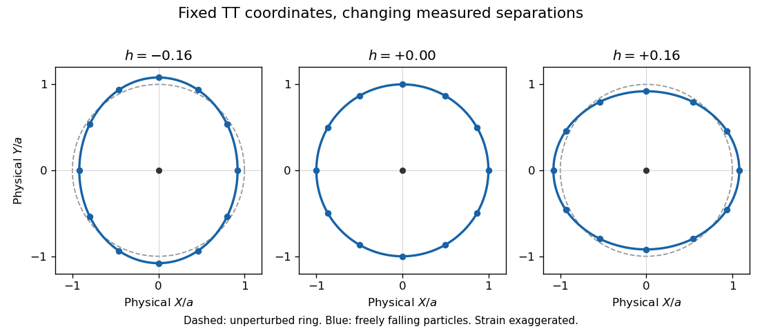
An observer at the center detects these changing distances, for example by exchanging light signals with the particles. Equivalently geodesic deviation gives the local tidal acceleration

\ddot{X} = \frac{1}{2} \ddot{h} X, \ddot{Y} = - \frac{1}{2} \ddot{h} Y

to the same order. There is physical relative motion and nonzero Riemann curvature tensor, even though the selected coordinate positions are constant. For a detector comparable to a wavelength, its light-travel-time response must be included rather than treating all distances as simultaneously measured local lengths.

d

Solution

Using the source's rounded solar mass, each hole has

m ≃ 3 \times 1 0^{31} kg

. Its Schwarzschild radius is

r_{s} = \frac{2 G m}{c ^{2}} ≃ \frac{2 ( 6.7 \times 1 0 ^{- 11} ) ( 3 \times 1 0 ^{31} )}{9 \times 1 0 ^{16}} ≃ 4.5 \times 1 0^{4} m .

Thus

r_{s} \sim 1 0^{5} m

at order-of-magnitude accuracy. Using the more accurate solar mass would give about

9 \times 1 0^{4} m

The stated orbit is not a consistent separated-hole weak-field binary. Its nominal center-to-center separation is only

20 km

, below even the above single-hole radius. Applying two isolated Schwarzschild spacetime descriptions and a circular Newtonian orbit at that separation is not controlled. Likewise an estimate

\overset{ˉ}{h}_{11}^{'} \sim r_{s} / r

r = 10 km

is of order one or larger, contradicting the small-perturbation assumption. The intended near-source statement is therefore a strong-field scale,

∣ \overset{ˉ}{h}_{11}^{'} ∣_{near} \sim 1,

not a reliable prediction from linearized gravity at the specified orbit. The exact radiative component is also gauge dependent near the source.

One can still estimate the intended distant gravitational wave strain scale. A radiative amplitude decreases as

1/ D

in the wave zone. A compact strong-field source has a characteristic length of order

r_{s}

, giving a dimensional strain estimate

h_{far} \sim r_{s} / D

, up to mass, orientation and efficiency factors of order unity. This is also the strong-field dimensional scale suggested by far-zone quadrupole strain; it is not an application of the slow-motion formula to the inconsistent orbit.

With the supplied conversion,

D = 500 \times 1 0^{6} \times 1 0^{16.5} m ≃ 1.6 \times 1 0^{25} m, h_{far} \sim \frac{4.5 \times 1 0 ^{4}}{1.6 \times 1 0 ^{25}} \sim 3 \times 1 0^{- 21} .

For a ring radius

a = 4 \times 1 0^{3} m

, part (c) gives a single principal semiaxis displacement amplitude

∣ δ a ∣ \sim \frac{a h _{far}}{2} \sim 6 \times 1 0^{- 18} m, of order 1 0^{- 18} - 1 0^{- 17} m .

The difference of the two principal semiaxes has twice this amplitude. This is a conditional dimensional estimate of a physically plausible merger signal at that distance; the supplied close circular orbit does not define a self-consistent waveform or a precise amplitude.

4

a

Solution

Normalize the present scale factor to

a_{0} = 1

. Conservation of the number of electrons associated with the baryons makes their physical number density scale as

a^{- 3}

. At this early epoch they are free rather than bound in neutral atoms, so

n_{e} = n_{e, 0} (\frac{a _{0}}{a})^{3} = 0.2 (1 0^{6})^{3} = 2 \times 1 0^{17} m^{- 3} .

Here the specified present density is interpreted as the conserved total electron abundance, including electrons that might be bound today. A present free-electron density would require an ionization-fraction correction.

Density alone does not determine whether a gas is relativistic; its random kinetic energy must be compared with the rest energy. In the usual thermal Hot Big Bang model, use the measured cosmic microwave background temperature

T_{0} ≃ 2.7 K

and the temperature scaling of thermal photon number and energy densities,

T_{γ} \propto a^{- 1}

. Tight coupling then gives

T_{e} ≃ T_{γ} ≃ 2.7 \times 1 0^{6} K, k_{B} T_{e} ≃ 230 eV .

Since

m_{e} c^{2} ≃ 5.1 \times 1 0^{5} eV

\frac{k _{B} T _{e}}{m _{e} c ^{2}} ≃ 4.5 \times 1 0^{- 4} ≪ 1 : the electrons are nonrelativistic .

Their thermal speed is of order

3 k_{B} T_{e} / m_{e} ≃ 0.04 c

. The gas is fully ionized because its temperature is far above the recombination temperature, but ionization does not imply relativistic electrons. Thermal electron-positron pairs are exponentially suppressed at this temperature.^[ref]

The given age and scale-factor ratio should be treated as independent supplied estimates in the following rate comparison. They do not describe the same epoch in standard radiation-era expansion:

a / a_{0} = 1 0^{- 6}

normally corresponds to an age of order a year, not

1 0^{4}

years. The density and temperature estimates above depend on the scale-factor ratio, not on assigning it the stated age.

b

Solution

For statistically independent Thomson scattering events, the probability of no scattering over a proper distance

s

exp (- n_{e} σ_{e} s)

. The photon mean free path in an ionized universe is therefore

ℓ_{γ} = \frac{1}{n _{e} σ _{e}} = \frac{1}{( 2 \times 1 0 ^{17} ) ( 6.7 \times 1 0 ^{- 29} )} ≃ 7.5 \times 1 0^{10} m .

This is about half an astronomical unit. It is a proper distance at that epoch, not a present-day comoving distance. The Thomson scattering approximation is appropriate because the electrons are nonrelativistic and typical photon energies are much smaller than

m_{e} c^{2}

. The source's spelling of the process is a typographical error; the physical process is Thomson scattering.

c

Solution

A photon travels at

c

, so its typical scattering interval is

t_{sc} = \frac{ℓ _{γ}}{c} ≃ \frac{7.5 \times 1 0 ^{10}}{3 \times 1 0 ^{8}} ≃ 2.5 \times 1 0^{2} s,

about four minutes. The supplied universe age is

t_{age} = 1 0^{4} yr ≃ 3.2 \times 1 0^{11} s .

Thus

\frac{t _{sc}}{t _{age}} ≃ 8 \times 1 0^{- 10}, \frac{t _{age}}{t _{sc}} \sim 1 0^{9} .

A photon scatters extremely frequently compared with the expansion timescale, of order the cosmic age. The plasma is opaque and its photons are tightly coupled to the electrons rather than freely streaming over a cosmological distance. In rate language

Γ_{γ} = n_{e} σ_{e} c ≫ H

, where

H

is the Hubble parameter.^[ref]

This is a statement about transport and momentum coupling. Elastic Thomson scattering alone does not create or destroy photons and hence is not, by itself, proof that an arbitrary photon spectrum reaches complete blackbody thermal equilibrium. The interaction interval calculated here is the interval experienced by a photon; the interval per electron differs because there are many more photons than electrons. Even replacing the inconsistent supplied age by the standard age of order a year at this scale factor would leave scattering much faster than expansion.

d

Solution

As the temperature falls, electrons and protons form neutral hydrogen through cosmological recombination. The free electron fraction drops sharply, and so does the scattering rate

Γ_{γ} = n_{e} σ_{T} c

. When this rate becomes comparable to or smaller than the Hubble parameter, the plasma becomes transparent and photon decoupling occurs. The Thomson scattering cross-section itself does not abruptly vanish. The rapid change is in the abundance of free targets.

The Hydrogen binding energy is

13.6 eV

, but recombination occurs at a much smaller thermal energy, of order

0.3 eV

, or a few thousand kelvin. There are roughly a billion photons per baryon, so the high-energy tail can keep hydrogen ionized long after

k_{B} T

drops below the binding energy. The falling exponential ionizing tail then makes the transition comparatively sharp. Last scattering follows when sufficiently few electrons remain free.^[ref]

To estimate a horizon, specify an expansion model as well as the redshift. The proper particle horizon at emission is

d_{ph} (t_{*}) = a (t_{*}) \int_{0}^{t_{*}} \frac{c d t}{a ( t )} .

As a transparent analytic estimate, approximate a spatially flat matter-dominated universe by

a (t) = (t / t_{now})^{2/3}

throughout. Then

d_{ph} (t_{*}) = 3 c t_{*}, t_{*} = \frac{t _{now}}{( 1 + z _{*} ) ^{3/2}} .

Taking the illustrative present value

H_{0} = 70 km s^{- 1} Mp c^{- 1}

, this model has

t_{now} = 2/ (3 H_{0}) ≃ 9.3 \times 1 0^{9} yr

. At

z_{*} = 1 0^{3}

t_{*} ≃ 3 \times 1 0^{5} yr, d_{ph} (t_{*}) ≃ 0.27 Mpc .

This is a proper horizon radius at emission; its corresponding present comoving length is about

270 Mpc

For the same model the comoving distance to the Cosmic microwave background last-scattering surface and its angular diameter distance are

χ_{*} = 3 c t_{now} [1 - (1 + z_{*})^{- 1/2}], D_{A} = \frac{χ _{*}}{1 + z _{*}} .

Therefore the angular extent associated with one radial horizon length is

θ_{ph} ≃ \frac{d _{ph}}{D _{A}} = \frac{1}{1 + z _{*} - 1} ≃ 0.033 rad ≃ 1. 9^{\circ} .

This is an order-one-degree estimate. Including the earlier radiation domination and late dark energy changes the coefficient; it does not make the horizon span the sky. A horizon patch diameter has twice this angle, whereas the acoustic scale uses a sound horizon and differs again. The redshift by itself, without an expansion model or normalization, is insufficient for a unique horizon distance.

The horizon problem is that the observed cosmic microwave background has nearly the same mean temperature across angular separations vastly greater than this scale. In the purely decelerating Hot Big Bang model, sufficiently separated last-scattering regions had neither time to exchange signals nor a common post-Big-Bang causal region that could establish their observed thermal uniformity. The puzzle concerns the missing causal explanation of those initial correlations; it is not an inconsistency of specifying uniform initial conditions mathematically. An earlier period of cosmic inflation can enlarge a formerly causally connected region beyond the later observable horizon.

2016 (A13484W1, B5)

Source paper: www.whatdotheyknow.com/request/physics_past_exam_papers_2015_16/response/973997/attach/3/Cowell%20Attachment.zip?cookie_passthrough=1. The dated cover identifies the Part B sitting of 18 June 2016. All four options are solved below.

1

Solution

Constants and radial motion. Write

m = GM / c^{2}

and

f (r) = 1 - 2 m / r

. A Schwarzschild black hole has spherical symmetry, so its conserved angular momentum fixes an orbital plane through the centre. A rotation of the angular coordinates puts any nonradial orbit in the equatorial plane. A radial orbit can also be placed in such a plane. This is a choice of coordinates, not a restriction on the possible orbital inclinations.

The quadratic geodesic Lagrangian, with a dot denoting differentiation with respect to the satellite's proper time, is

L = \frac{1}{2} [- f c^{2} \dot{t}^{2} + f^{- 1} \overset{r}{˙}^{2} + r^{2} \dot{ϕ}^{2}] = - \frac{c ^{2}}{2} .

The last equality is four-velocity normalization, imposed after deriving the Euler-Lagrange equations. The cyclic coordinates

t, ϕ

give independent conserved specific Killing energy and angular momentum:

e = f \dot{t}, ℓ = r^{2} \dot{ϕ}, \dot{t} = \frac{e}{f}, \dot{ϕ} = \frac{ℓ}{r ^{2}} .

Here

e

is the conserved energy per unit rest energy and

ℓ

has dimensions of angular momentum per unit mass. Substituting them in the normalization condition gives

\overset{r}{˙}^{2} = c^{2} e^{2} - f (c^{2} + \frac{ℓ ^{2}}{r ^{2}}) = c^{2} (e^{2} - 1) + \frac{2 GM}{r} - \frac{ℓ ^{2}}{r ^{2}} + \frac{2 GM ℓ ^{2}}{c ^{2} r ^{3}} .

The two signs of

\overset{r}{˙}

distinguish outgoing and ingoing branches; the expression must be nonnegative on the allowed radial interval.

For a nonradial orbit, put

u = 1/ r

. Since

\overset{r}{˙} = - ℓ d u / d ϕ

, the radial equation becomes

(\frac{d u}{d ϕ})^{2} = \frac{c ^{2} ( e ^{2} - 1 )}{ℓ ^{2}} + \frac{2 GM}{ℓ ^{2}} u - u^{2} + 2 m u^{3} .

Differentiating and extending continuously through isolated radial turning points gives

\frac{d ^{2} u}{d ϕ ^{2}} + u = \frac{GM}{ℓ ^{2}} + \frac{3 GM}{c ^{2}} u^{2}, A = \frac{GM}{ℓ ^{2}}, B = \frac{3 GM}{c ^{2}} .

A circular solution can equivalently be obtained directly from the radial geodesic equation, avoiding division by

d u / d ϕ = 0

everywhere on that special orbit.

Circular launch and the station's clock. For

u = 1/ R

the orbit equation gives

ℓ_{c}^{2} = \frac{GMR}{1 - 3 m / R}, e_{c} = \frac{1 - 2 m / R}{1 - 3 m / R}, Ω = \frac{d ϕ}{d t} = \frac{GM}{R ^{3}} .

The static astronaut measures circumferential proper length

R d ϕ

and station proper time

d τ_{s} = f (R) d t

. Thus the Schwarzschild circular-orbit local speed and return time are

v_{circ} = \frac{R Ω}{f ( R )} = \frac{GM}{R - 2 GM / c ^{2}}, Δ τ_{s} = 2 π \frac{R ^{3}}{GM} 1 - \frac{2 GM}{c ^{2} R} .

This is a local speed measured with the astronaut's clock, not the satellite's proper velocity

γ v

. After one azimuthal revolution the circular satellite meets the fixed station again. For comparison, the satellite's own elapsed proper time would instead be

2 π R^{3} / (GM) 1 - 3 m / R

A static station requires

R > 2 m

; a timelike circular satellite requires

R > 3 m

, since the local circular speed must be below

c

. The circular orbit is stable only for

R > 6 m

, marginal at

6 m

, and unstable for

3 m < R < 6 m

. Thus a request for a robust near-circular trajectory implicitly needs more than merely placing the station outside the horizon.

Slightly changing the launch speed. In the stable, bound regime, a small tangential increase makes the launch point a pericentre; a small decrease makes it an apocentre, provided the perturbed orbit remains outside its plunge separatrix. In either case the orbit is a precessing rosette, not an exactly closed Newtonian ellipse. For an explicit first-order description write

A = A_{c} + δ A

and

u = 1/ R + δ u

. Then

δ u^{''} + κ_{ϕ}^{2} δ u = δ A, κ_{ϕ}^{2} = 1 - \frac{6 m}{R}, δ u = \frac{δ A}{κ _{ϕ}^{2}} [1 - cos (κ_{ϕ} ϕ)] .

The tangential launch gives

δ u (0) = δ u^{'} (0) = 0

. At the station,

ℓ = R γ v

, so

δ ℓ / ℓ_{c} = γ_{c}^{2} Δ v / v_{circ}

and

δ A = - 2 A_{c} γ_{c}^{2} Δ v / v_{circ}

. Therefore

r - R ≃ \frac{2 ( R - 2 m )}{1 - 6 m / R} \frac{Δ v}{v _{circ}} [1 - cos (κ_{ϕ} ϕ)] .

This perturbative expression also requires the resulting radial excursion to be small compared with

R

; close to the innermost stable orbit,

∣Δ v ∣ ≪ v_{circ}

alone does not ensure that.

The Schwarzschild launch-orbit recurrence needs care when deciding whether a collision is inevitable. The satellite returns to radius

R

once per radial cycle, after an azimuthal advance approximately

Φ_{r} = 2 π / κ_{ϕ}

. It returns to the station's exact point only if an integer number of radial cycles also gives an integer number of azimuthal revolutions. Rational

Φ_{r} / (2 π)

gives an exact return; an irrational ratio gives arbitrarily close approaches but no exact post-launch return for ideal point objects. At

R = 12 m

, for example, the linearized ratio is

2

, illustrating why precession alone does not prove an exact collision. For generic bound orbits the dense recurrence eventually threatens any station and satellite of nonzero size; a resonant closed rosette returns exactly. A small speed adjustment is therefore not a robust permanent collision-avoidance manoeuvre for a bound satellite.

There is no unconditional collision conclusion without specifying the regime. An unstable circular orbit cannot support the small bounded oscillations used above. In particular, near

R = 3.5 m

the circular specific energy is already

e_{c} > 1

; a small positive speed increment can send the satellite outward on an unbound escape orbit, with no subsequent return to

R

. Such an escape is a different way to avoid a future encounter. Radiation reaction and manoeuvres have been excluded throughout the ideal test-particle calculation.

Figure 1.
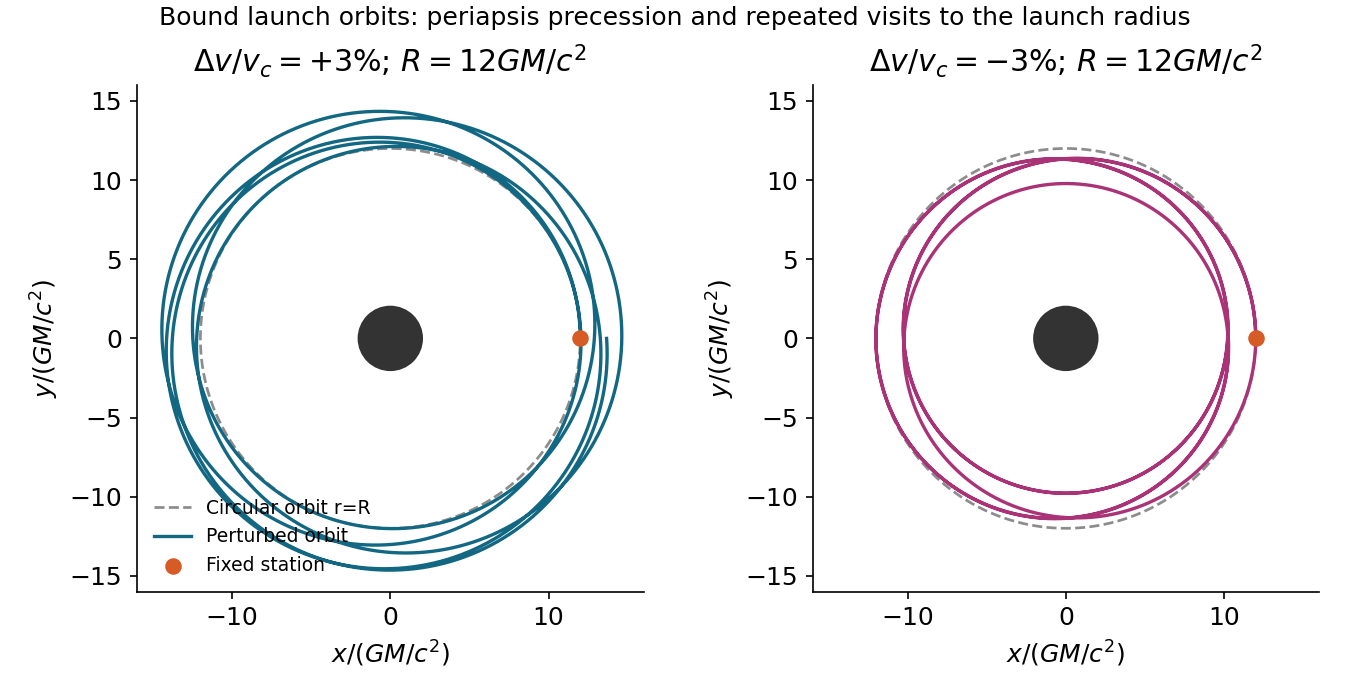
Bound Schwarzschild trajectories after small positive and negative tangential launch-speed changes
. **Details**.

2

Solution

Curvature and conservation. The stress-energy tensor is symmetric and obeys covariant conservation of stress-energy,

\nabla_{a} T^{ab} = 0

. To construct a local field equation linear in the Ricci tensor and its trace, consider

R^{ab} + α g^{ab} R

. The contracted Bianchi identity and metric compatibility give

\nabla_{a} R^{ab} = \frac{1}{2} \nabla^{b} R, \nabla_{a} (R^{ab} + α g^{ab} R) = (\frac{1}{2} + α) \nabla^{b} R .

The divergence must vanish identically, rather than constrain every matter source to have constant scalar curvature. Therefore

α = - 1/2

, giving the Einstein tensor

G^{ab} = R^{ab} - \frac{1}{2} g^{ab} R, \nabla_{a} G^{ab} = 0 .

A constant multiple of the metric can also be added, corresponding to a cosmological constant; it is omitted in this stellar problem. Proportionality to matter by itself does not exclude arbitrary higher-curvature theories. The stated linear combination assumes the usual second-order metric field equation, linear in curvature, with its coupling fixed by the Newtonian limit.

The source's displayed curvature components use the convention

G_{ab} = - 8 π G T_{ab} / c^{4}

, opposite to another common curvature convention. Retain both that sign and those components together: replacing only the sign would give an incorrect negative stellar mass.

Fluid frame and mass function. Because the metric and the Einstein tensor are diagonal, the mixed time-space components of the stress-energy tensor vanish. For the perfect fluid in general relativity,

T^{0 i} = (ρ + p / c^{2}) u^{0} u^{i}

. A future timelike four-velocity has

u^{0} \neq = 0

, so ordinary matter with

ρ c^{2} + p \neq = 0

must have

u^{i} = 0

. Normalizing

g_{ab} u^{a} u^{b} = - c^{2}

then yields

u^{0} = c e^{- Φ}, u_{0} = - c e^{Φ} .

The static perfect-fluid rest-frame criterion needs the nonzero enthalpy assumption. A vacuum-like component with

p = - ρ c^{2}

has

T^{ab} = p g^{ab}

for every normalized timelike

u^{a}

, so diagonality cannot pick its rest frame. That is a concrete exception to the unqualified inference about velocity; it does not describe the ordinary stellar fluid considered next.

Lowering the indices of the static-fluid tensor gives

T_{00} = ρ c^{2} e^{2Φ}

and

T_{11} = p e^{2Λ}

. The time component of the field equation therefore implies

\frac{d}{d r} [r (1 - e^{- 2Λ})] = \frac{8 π G}{c ^{2}} ρ r^{2} = \frac{2 G}{c ^{2}} \frac{d M}{d r} .

Regularity at the centre fixes the integration constant to zero, giving

e^{- 2Λ (r)} = 1 - \frac{2 GM ( r )}{c ^{2} r}, Λ (r) = - \frac{1}{2} ln (1 - \frac{2 GM ( r )}{c ^{2} r}) .

A central point mass would introduce an additional constant, but is excluded by the regular-star boundary condition. The radial field equation is

\frac{e ^{2Λ} - 1}{r ^{2}} - \frac{2 Φ ^{'}}{r} = - \frac{8 π G}{c ^{4}} p e^{2Λ} .

Solving and substituting the mass function gives

Φ^{'} = \frac{G [ M ( r ) + 4 π p r ^{3} / c ^{2} ]}{c ^{2} r ^{2} [ 1 - 2 GM ( r ) / ( c ^{2} r )]} .

Combining this with fluid conservation gives the Tolman–Oppenheimer–Volkoff equation, in conventions where

ρ

is the rest-frame mass-equivalent energy density:

\frac{d p}{d r} = - \frac{G ( ρ + p / c ^{2} ) [ M ( r ) + 4 π p r ^{3} / c ^{2} ]}{r ^{2} [ 1 - 2 GM ( r ) / ( c ^{2} r )]}, M^{'} = 4 π ρ r^{2} .

The pressure contributes to inertial mass density and active gravity, while the last denominator is a relativistic curvature correction. The weak-field, low-pressure limit recovers

p^{'} ≃ - GρM / r^{2}

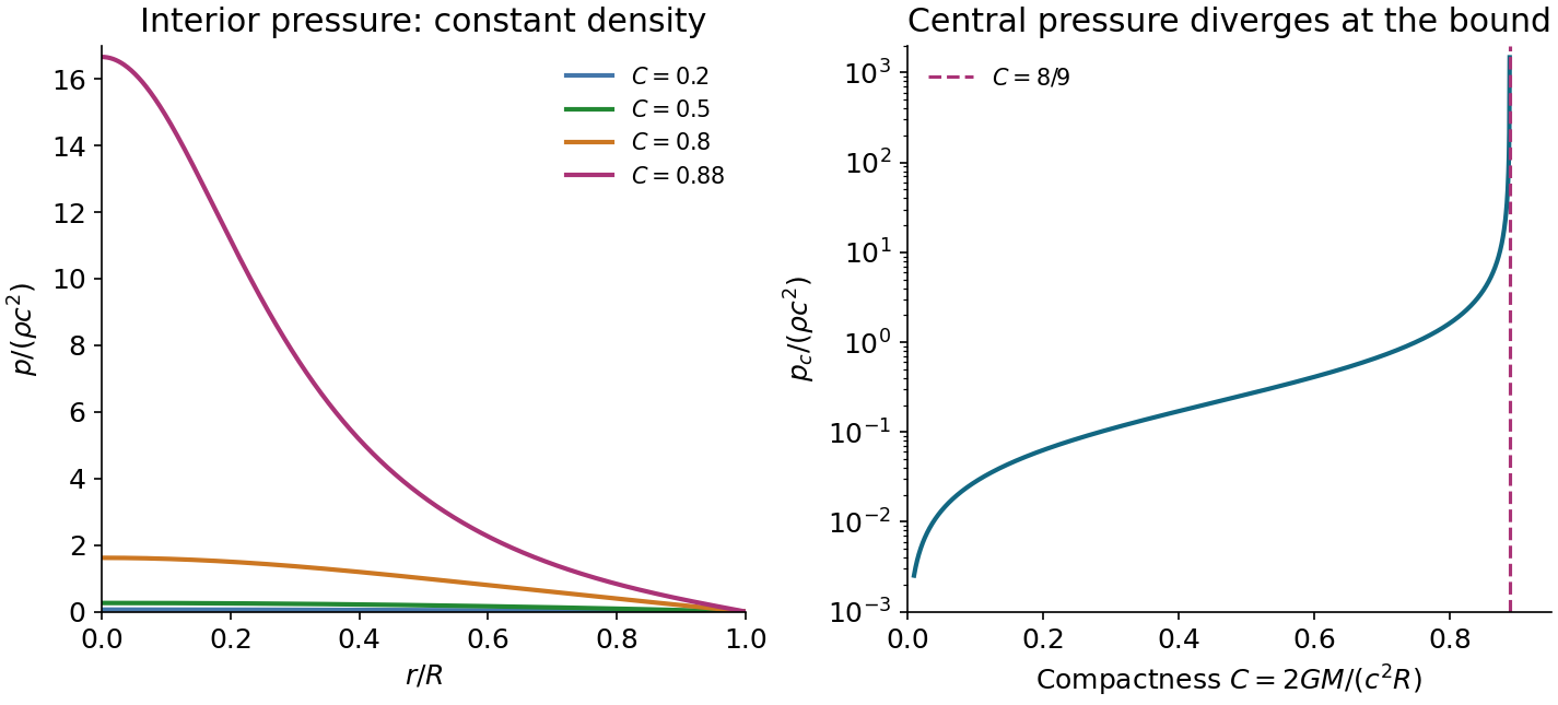
Constant-density integration. Set

w = p / (ρ c^{2})

and

α = 8 π Gρ / (3 c^{2})

. Now

M (r) = 4 π ρ r^{3} /3

and

\frac{d w}{( 1 + w ) ( 1 + 3 w )} = - \frac{α}{2} \frac{r d r}{1 - α r ^{2}} .

The surface boundary condition is

p (R) = 0

, with finite central pressure. Integrating from the surface gives

\frac{1}{2} ln \frac{1 + 3 w}{1 + w} = \frac{1}{4} ln \frac{1 - α r ^{2}}{1 - α R ^{2}} .

(10)

Write

s (r) = 1 - 2 GM r^{2} / (c^{2} R^{3})

and

s_{R} = 1 - 2 GM / (c^{2} R)

. Solving for

w

gives the Interior Schwarzschild solution:

p (r) = ρ c^{2} \frac{s ( r ) - s _{R}}{3 s _{R} - s ( r )}, p_{0} = ρ c^{2} \frac{1 - s _{R}}{3 s _{R} - 1} .

(11)

The printed integration hint has a missing factor for general

A

. The common-intercept partial fraction identity gives

\frac{1}{( A + 3 x ) ( A + x )} = \frac{1}{2 A} [\frac{3}{A + 3 x} - \frac{1}{A + x}] (A \neq = 0) .

(12)

For instance, at

A = 2, x = 0

the integrand on the left is

1/4

, while the derivative of the printed right-hand side is

1/2

. The normalized

w

calculation above uses

A = 1

, where that missing factor happens not to matter.

Positive finite central pressure requires

3 s_{R} > 1

. Consequently

\frac{2 GM}{c ^{2} R} < \frac{8}{9}, M < \frac{4 c ^{2} R}{9 G} .

(13)

Equality is a singular limiting solution with divergent pressure. The constant-density model is incompressible and is not a realistic causal neutron-star equation of state. Nevertheless, Buchdahl's theorem extends this compactness bound to regular static spherical isotropic fluids with nonincreasing density, under its usual assumptions.

For an emitted surface line received by a static observer at infinity, the gravitational redshift between static Schwarzschild observers gives

1 + z = (1 - \frac{2 GM}{c ^{2} R})^{- 1/2} < 3, z < 2 .

(14)

A claimed purely gravitational surface redshift

z = 3.1

would require compactness

1 - 1/ (4.1)^{2} ≃ 0.9405

, exceeding

8/9

. It is inconsistent with the regular isotropic static neutron-star interpretation, even though the surface would formally remain outside its Schwarzschild radius. Misidentification, additional kinematic shifts or departures from the model would need examination before treating that line as a neutron-star surface measurement.

Figure 1.
Constant-density relativistic pressure profiles and the divergence at the compactness bound
. **Details**.

3

Solution

Spatial geometry. An embedding of the three-sphere is

w = A cos χ, z = A sin χ cos θ, x = A sin χ sin θ cos ϕ, y = A sin χ sin θ sin ϕ .

Taking differentials and collecting terms gives the induced metric tensor

d ℓ^{2} = A^{2} d χ^{2} + A^{2} sin^{2} χ (d θ^{2} + sin^{2} θ d ϕ^{2}) .

Put

\overset{r}{ˉ} = A sin χ

. Then

d \overset{r}{ˉ} = A cos χ d χ

, so

d ℓ^{2} = \frac{d r ˉ ^{2}}{1 - r ˉ ^{2} / A ^{2}} + \overset{r}{ˉ}^{2} d Ω^{2}, d Ω^{2} = d θ^{2} + sin^{2} θ d ϕ^{2} .

The areal radius

\overset{r}{ˉ}

is not a global radial coordinate on the entire three-sphere: its maximum occurs at the equator and two hemispheres share each smaller value. Use separate charts there; the coordinate singularity at

\overset{r}{ˉ} = A

is not a physical singularity.

For Euclidean space and hyperbolic space of curvature

- 1/ A^{2}

, respectively,

d ℓ_{0}^{2} = d \overset{r}{ˉ}^{2} + \overset{r}{ˉ}^{2} d Ω^{2}, d ℓ_{-}^{2} = \frac{d r ˉ ^{2}}{1 + r ˉ ^{2} / A ^{2}} + \overset{r}{ˉ}^{2} d Ω^{2} .

For the latter,

\overset{r}{ˉ} = A sinh χ

gives

d ℓ_{-}^{2} = A^{2} [d χ^{2} + sinh^{2} χ d Ω^{2}]

. In all three cases the induced two-metric at fixed

\overset{r}{ˉ} = \overset{ˉ}{R}

\overset{ˉ}{R}^{2} d Ω^{2}

. Its surface area is therefore

A (\overset{ˉ}{R}) = \int_{0}^{2 π} d ϕ \int_{0}^{π} \overset{ˉ}{R}^{2} sin θ d θ = 4 π \overset{ˉ}{R}^{2} .

This equality compares the same areal radius, not the same proper radial distance. For a proper radial distance

ℓ

, the corresponding areas are

4 π A^{2} sin^{2} (ℓ / A)

4 π ℓ^{2}

, and

4 π A^{2} sinh^{2} (ℓ / A)

Homogeneity, isotropy and redshift. The FRW metric has constant-time spatial slices of constant curvature

k / a^{2} (t)

, with

k = + 1, 0, - 1

selecting the three geometries above. Their isometries act transitively on points and isotropically about every point, implementing the cosmological principle. Multiplication by one common time-dependent scale factor preserves these properties. With the source's

k = \pm 1

normalization,

r

is dimensionless and

a

has units of length; using a dimensionless scale factor instead rescales the spatial curvature parameter. The origin of the spherical coordinates is arbitrary; it does not identify a physical centre. Cosmic time is the proper time of the comoving observers, and the absence of time-space cross terms makes their worldlines orthogonal to the homogeneous slices.

For a radial null geodesic between comoving endpoints,

\int_{t_{E}}^{t_{0}} \frac{c d t}{a ( t )} = \int_{0}^{R} \frac{d r}{1 - k r ^{2}} .

The next wave crest travels between the same endpoints. Subtracting the two path integrals, for wave periods short compared with the expansion time, gives

δ t_{0} / a_{0} = δ t_{E} / a_{E}

. Thus the cosmological redshift is

1 + z = \frac{λ _{0}}{λ _{E}} = \frac{ν _{E}}{ν _{0}} = \frac{a _{0}}{a _{E}} .

Both observers' clocks are cosmic proper-time clocks. Peculiar velocities and local gravitational-potential shifts have been left out of this homogeneous calculation.

Angular size and brightness. For a galaxy small compared with its distance, the angular diameter distance is

D_{A} = a_{E} R

and its angular diameter is

Δ θ ≃ \frac{d}{a _{E} R} = \frac{( 1 + z ) d}{a _{0} R} .

Here the emitted proper diameter is measured transverse to the line of sight; radial proper distance is a different integral when

k \neq = 0

. Ignoring absorption, lensing caustics and intrinsic evolution, photon-number conservation spreads an isotropic-equivalent luminosity across the sphere

4 π a_{0}^{2} R^{2}

. Each photon loses energy by

1 + z

, and its arrival interval is stretched by the same factor. The received bolometric flux is

F = \frac{L}{4 π a _{0}^{2} R ^{2} ( 1 + z ) ^{2}}, D_{L} = (1 + z) a_{0} R = (1 + z)^{2} D_{A} .

The disc's proper projected area is

A_{d} = π d^{2} /4

, and its observed solid angle is

Ω_{d} ≃ A_{d} / D_{A}^{2}

. Therefore its surface brightness is

I_{obs} = \frac{F}{Ω _{d}} = \frac{L}{4 π A _{d}} (1 + z)^{- 4} = \frac{L}{π ^{2} d ^{2}} (1 + z)^{- 4} .

(10)

This is cosmological surface-brightness dimming. The normalization uses

L

as isotropic-equivalent luminosity along the viewing direction; another disc emission law changes that normalization but not the redshift power. This is a bolometric result. In a specified observed frequency band the emitted spectrum is sampled at a shifted frequency and requires a spectral correction.

The distinction in telescope aperture and resolved surface brightness matters here. A larger telescope collects more photons and improves angular resolution, but cannot restore the incoming radiance lost by cosmological dimming. For aperture diameter

D

and a diffraction resolution element of solid angle

Ω_{res} \sim (λ / D)^{2}

, the collected power from uniform resolved brightness scales as

I_{obs} A_{tel} Ω_{res} \propto I_{obs} λ^{2},

(11)

independent of

D

. This is consistent with conservation of etendue. It explains why increasing aperture while keeping every gain in resolution does not increase counts per native resolution element from a smooth extended source. It does not make larger telescopes useless: at a fixed angular bin the counts grow as

D^{2}

, so a photon-noise-limited or uniform-sky-noise-limited signal-to-noise ratio grows roughly as

D t_{exp}

. They also resolve smaller structures and improve point-source sensitivity. Aperture, exposure and angular binning help measure a dim galaxy, without changing its intrinsic

(1 + z)^{- 4}

brightness penalty.

Figure 1.
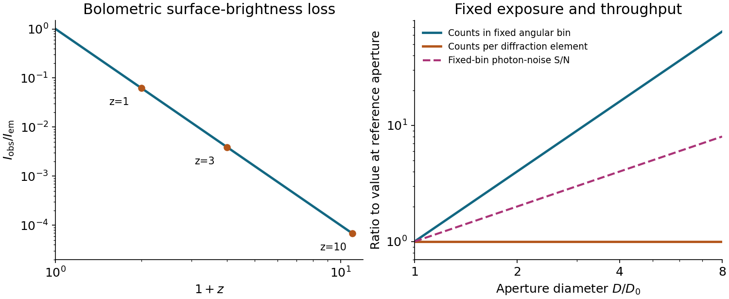
Cosmological surface-brightness dimming and the distinct aperture scalings of fixed angular bins and diffraction elements
. **Details**.

4

Solution

Two stages of the thermal history. Big Bang nucleosynthesis is nuclear assembly in an almost fully ionized, radiation-dominated plasma. Around

t \sim 1 s

, at temperatures of order

1 MeV / k_{B}

, the weak neutron–proton conversion rate falls below the expansion rate. The neutron-to-proton abundance freezes out at order

1/5

and then decreases by neutron decay. The deuterium bottleneck delays effective nuclear assembly until

k_{B} T \sim 0.07

–

0.1 MeV

, at ages of a few minutes: the high photon-to-baryon ratio permits photodissociation despite the deuteron binding energy exceeding the mean photon energy. Once deuterium survives, reactions rapidly put most remaining neutrons into helium-4. A neutron-to-proton ratio near

1/7

gives a helium mass fraction

Y_{p} ≃ 2 (n / p) / (1 + n / p) ≃ 1/4

, with hydrogen dominant by number and small residual deuterium, helium-3 and lithium-7 abundances. Expansion and low density prevent substantial heavy-element production. Nuclear binding is involved; neutral atoms do not yet survive.

Photon decoupling occurs much later, near a few thousand kelvin and a few hundred thousand years, after matter has overtaken radiation in the expansion dynamics. Electrons and nuclei form neutral atoms during cosmological recombination. The resulting decline of free-electron density reduces Thomson opacity, and photons begin to free stream over cosmological distances. Those photons form the observed cosmic microwave background. Atomic binding and scattering opacity, rather than new nuclear reactions, control this stage. Helium forms neutral atoms earlier than hydrogen. Recombination, photon last scattering, baryon drag release and the later thermal decoupling of the gas are related but not identical events.

The temperature falls through expansion: after the relevant entropy releases have ended,

T_{γ} \propto a^{- 1}

and number densities scale as

a^{- 3}

. Big Bang nucleosynthesis lies in the radiation-dominated universe; photon decoupling lies after matter–radiation equality, when a matter-dominated approximation is useful but radiation is not exactly negligible.

Photon density and baryon abundance. The cosmic microwave background has a black-body radiation spectrum obeying Planck's law:

u_{ν} = \frac{8 πh ν ^{3}}{c ^{3}} \frac{1}{e ^{h ν / (k_{B} T)} - 1}, T_{0} ≃ 2.725 K,

where

u_{ν}

is spectral energy density, not a photon-number density. The measured temperature is about

2.72548 K

.^[ref] The mean photon energy in a black body is

⟨ E_{γ} ⟩ = \frac{π ^{4}}{30 ζ ( 3 )} k_{B} T ≃ 2.701 k_{B} T .

Using the supplied rounded energy density gives

n_{γ 0} ≃ \frac{4 \times 1 0 ^{- 14}}{2.701 k _{B} T _{0}} ≃ 3.9 \times 1 0^{8} m^{- 3} .

The exact black-body number integral at

2.725 K

gives

4.1 \times 1 0^{8} m^{- 3}

; the difference reflects rounding of the stated energy density. Either estimate is adequate.

A numerical photon-to-baryon ratio additionally needs a baryon density, which is not printed in this question. Make that observational input explicit rather than infer baryons from radiation alone. For illustration take the standard rounded physical density

Ω_{b} h_{H}^{2} ≃ 0.022

, with

H_{0} = 100 h_{H} km s^{- 1} Mp c^{- 1}

. This is consistent with the cosmological parameter fits available around the paper's date.^[ref] It gives

ρ_{b 0} = (Ω_{b} h_{H}^{2}) \frac{3 ( 100 km s ^{- 1} Mp c ^{- 1} ) ^{2}}{8 π G} ≃ 4.1 \times 1 0^{- 28} kg m^{- 3}, n_{b 0} ≃ \frac{ρ _{b 0}}{m _{p}} ≃ 0.25 m^{- 3} .

Counting baryons, including those bound in helium, rather than counting nuclei then gives

\frac{n _{γ}}{n _{b}} \sim 1.6 \times 1 0^{9}, η \equiv \frac{n _{b}}{n _{γ}} \sim 6 \times 1 0^{- 10} .

Both populations dilute as

a^{- 3}

after electron–positron annihilation, so this ratio also applies at hydrogen recombination in the standard adiabatic history.

Estimating decoupling. The large photon excess explains why setting

k_{B} T

equal to the Hydrogen binding energy

χ_{H} = 13.6 eV

is wrong. Even a small ionizing tail can oppose neutral-atom formation. The crude exponential balance

e^{- χ_{H} / (k_{B} T)} \sim η

gives

χ_{H} / (k_{B} T) \sim ln (1/ η) \sim 21

, or

T \sim 7 \times 1 0^{3} K

. This only establishes the scale and the large suppression below

χ_{H} / k_{B}

; it neglects phase-space factors and the opacity criterion.

A more controlled elementary Saha-Thomson decoupling estimate uses the hydrogen-only Saha equation. With

X_{e} = n_{e} / n_{H}

and ground-state statistical weights combined in the usual way,

\frac{X _{e}^{2}}{1 - X _{e}} = \frac{1}{n _{H}} (\frac{2 π m _{e} k _{B} T}{h ^{2}})^{3/2} e^{- χ_{H} / (k_{B} T)}, n_{H} ≃ (1 - Y_{p}) n_{b 0} (\frac{T}{T _{0}})^{3} .

The electron translational phase-space factor is significant inside the logarithm. This equilibrium relation places the sharp neutralization interval around

T \sim (3 - 4) \times 1 0^{3} K

. Combine it with the approximate Thomson decoupling rate criterion

Γ_{γ} = n_{e} σ_{T} c \sim H, H ≃ H_{0} Ω_{m} (\frac{T}{T _{0}})^{3/2} .

For

Y_{p} ≃ 0.25

n_{b 0} ≃ 0.25 m^{- 3}

H_{0} ≃ 68 km s^{- 1} Mp c^{- 1}

, and

Ω_{m} ≃ 0.31

, solving these two approximate relations gives

T ≃ 3.1 \times 1 0^{3} K

, with equilibrium

X_{e}

of order

1 0^{- 2}

. Thus the appropriate estimate is

T_{dec} \sim 3 \times 1 0^{3} K, k_{B} T_{dec} \sim 0.26 eV, z_{dec} \sim 1100 .

This is not a precision recombination calculation. Hydrogen-only equilibrium omits the kinetic bottleneck in escaping Lyman photons, two-photon processes, the detailed helium history and freeze-out;

Γ/ H \sim 1

is not identical to the maximum of the last-scattering visibility function. These approximations must be improved to predict an accurate free-electron fraction or a percent-level last-scattering redshift. The high photon-to-baryon ratio alone does not fix that detailed history.

The electrons are highly nonrelativistic:

k_{B} T / (m_{e} c^{2}) \sim 5 \times 1 0^{- 7}

, and their thermal root-mean-square speed is only about

1 0^{- 3} c

. Photon coupling does not make their kinetic energies relativistic.

Age–temperature relation. During a nearly flat pressureless matter-dominated phase, with radiation, curvature and vacuum energy neglected in the expansion equation,

ρ_{m} \propto a^{- 3}, (\frac{a ˙}{a})^{2} \propto a^{- 3}, a (t) \propto t^{2/3} .

Here the Big Bang time is chosen as

t = 0

. Conserved photon entropy gives

T \propto a^{- 1}

, so

T \propto t^{- 2/3}, t \propto T^{- 3/2} .

(10)

To normalize this relation, use the matter-era expansion rate expressed in present-day measured parameters, rather than assume the late universe is still matter dominated:

t (T) ≃ \frac{2}{3 H _{0} Ω _{m}} (\frac{T _{0}}{T})^{3/2} .

(11)

The same illustrative parameters give

t_{dec} \sim 4.5 - 5 \times 1 0^{5} yr

for

T_{dec} \sim 3.0 - 3.1 \times 1 0^{3} K

. Radiation was still a meaningful correction; retaining it reduces the age, and a more complete recombination calculation gives the familiar scale of roughly

4 \times 1 0^{5} yr

.^[ref] A numerical age cannot follow from a proportionality

t \propto T^{- 3/2}

alone: an expansion or density normalization is essential. The small amount of dark energy at decoupling can be neglected even though it affects the present age.

2015 (A13484W1, B5)

Source paper: www-thphys.physics.ox.ac.uk/people/AndreiStarinets/TUTORIALS_NOTES_GR/gr_cosmology_exam_paper_2015.pdf

Worked answers: www-thphys.physics.ox.ac.uk/people/AndreiStarinets/TUTORIALS_NOTES_GR/gr-cosmology-exam-paper-2015-solutions.pdf

Oxford publishes matching worked answers for the complete held paper. New solutions are skipped.

2014 draft 2018-12-03 (A13484W1, B5)

Source paper: www-thphys.physics.ox.ac.uk/people/AndreiStarinets/TUTORIALS_NOTES_GR/gr_cosmology_exam_paper_2019.pdf

Worked answers: www-thphys.physics.ox.ac.uk/people/AndreiStarinets/TUTORIALS_NOTES_GR/gr-cosmology-exam-paper-2019-solutions.pdf

Oxford publishes matching worked answers for the complete held paper. New solutions are skipped.

The cover says 2014 and the document is stamped “DRAFT December 3, 2018”. Oxford links this exact document as its 2019 question paper, with matching answers. It contains different questions from the original 2014 paper and is kept separate.

2014 (2705, B5)

Source paper: www-thphys.physics.ox.ac.uk/people/AndreiStarinets/TUTORIALS_NOTES_GR/gr_cosmology_exam_paper_2014.pdf

Worked answers: www-thphys.physics.ox.ac.uk/people/AndreiStarinets/TUTORIALS_NOTES_GR/gr-cosmology-exam-paper-2014-solutions.pdf

Oxford publishes matching worked answers for the complete held paper. New solutions are skipped.

2013 (2764, B3: V)

Source paper: www-thphys.physics.ox.ac.uk/people/AndreiStarinets/TUTORIALS_NOTES_GR/gr_cosmology_exam_paper_2013.pdf

The lettered subdivisions index the successive separately marked blocks of each source question.

(-, +, +, +)

x^{0} = c t

, and retain terms linear in

Φ/ c^{2}

Ψ/ c^{2}

. The inverse metric is

g^{00} = - (1 - 2Φ/ c^{2})

and

g^{ij} = (1 + 2Ψ/ c^{2}) δ^{ij}

. In the Christoffel symbol formula

Γ^{α}_{β γ} = \frac{1}{2} g^{α δ} (\partial_{β} g_{δ γ} + \partial_{γ} g_{δ β} - \partial_{δ} g_{β γ}),

the differentiated metric perturbation is already first order, so the prefactor can be replaced by the flat inverse metric. For example

Γ^{0}_{ij} = \frac{1}{2} \partial_{0} g_{ij} = - δ_{ij} \partial_{0} Ψ/ c^{2}

and

Γ^{k}_{00} = - \frac{1}{2} \partial_{k} g_{00} = \partial_{k} Φ/ c^{2}

. Evaluating the remaining components gives

Γ^{0}_{00} Γ^{k}_{00} = \frac{\partial _{0} Φ}{c ^{2}}, = \frac{\partial _{k} Φ}{c ^{2}}, Γ^{0}_{0 i} Γ^{k}_{0 i} = \frac{\partial _{i} Φ}{c ^{2}}, = - \frac{\partial _{0} Ψ}{c ^{2}} δ_{i}^{k}, Γ^{0}_{ij} Γ^{k}_{ij} = - \frac{\partial _{0} Ψ}{c ^{2}} δ_{ij}, = - \frac{\partial _{i} Ψ δ _{j}^{k} + \partial _{j} Ψ δ _{i}^{k} - \partial ^{k} Ψ δ _{ij}}{c ^{2}} .

The lower-index symmetry follows from the torsion-free connection. Products of these first-order Christoffel symbols are beyond the retained weak-field approximation.

b

Solution

A pressureless relativistic fluid has stress-energy tensor

T^{μν} = ρ u^{μ} u^{ν}

, with four-velocity normalized by

u^{μ} u_{μ} = - c^{2}

. In its rest frame,

u^{i} = 0

, so

T^{0}_{0} = - ρ c^{2}, T^{i}_{j} = 0

. Here

ρ

is rest-frame mass density, or energy density divided by

c^{2}

For the linearized Ricci tensor and scalar, discard the quadratic connection terms. The contracted connection is

Γ^{μ}_{μν} = \partial_{ν} (Φ - 3Ψ) / c^{2}

. Differentiation then gives

R_{00} R_{0 i} R_{ij} R = \frac{\nabla ^{2} Φ + 3 \partial _{0}^{2} Ψ}{c ^{2}}, = \frac{2 \partial _{0} \partial _{i} Ψ}{c ^{2}}, = \frac{\partial _{i} \partial _{j} ( Ψ - Φ ) + δ _{ij} ( \nabla ^{2} Ψ - \partial _{0}^{2} Ψ )}{c ^{2}}, = \frac{4 \nabla ^{2} Ψ - 2 \nabla ^{2} Φ - 6 \partial _{0}^{2} Ψ}{c ^{2}} .

The Ricci scalar uses the zeroth-order inverse metric,

R = - R_{00} + δ^{ij} R_{ij}

, because multiplying first-order curvature by another metric perturbation would again be second order. These are the linearized curvature of a two-potential weak-field metric in the paper's Riemann curvature tensor sign convention.

c

Solution

The Einstein tensor is

G^{μ}_{ν} = R^{μ}_{ν} - \frac{1}{2} δ_{ν}^{μ} R

. Thus

G^{0}_{0} = - R_{00} - R /2

, where the time raising introduces the minus sign. Substitution cancels the

Φ

and time-derivative terms in that component and gives

G^{0}_{0} G^{i}_{j} = - \frac{2 \nabla ^{2} Ψ}{c ^{2}} = - \frac{8 π Gρ}{c ^{2}}, = \frac{2 \partial _{0}^{2} Ψ δ _{j}^{i} + \nabla ^{2} ( Φ - Ψ ) δ _{j}^{i} + \partial ^{i} \partial _{j} ( Ψ - Φ )}{c ^{2}} = 0.