Past exam of the mathematical methods II course of the University of Oxford / 2014 (4296, CP4)

Source: public Oxford archive. The held cover dates this ordinary sitting to 12 June 2014. Separate unlettered marked blocks are indexed a, b and so on; all Section B options are answered.

Stokes theorem gives ${\int }_S(\nabla \times \mathbf{F})\cdot \hat{\mathbf{n}}dS={\oint }_{\partial S}\mathbf{F}\cdot d\mathbf{r}$ for a sufficiently smooth vector field and consistently oriented surface and boundary. Choose the hemisphere's outward normal vector; its boundary circle is then traversed counterclockwise viewed from $+z$. Parametrize it by $\mathbf{r}=(2\cos t,2\sin t,0)$, $0\le t\le 2\pi$. On this curve, $\mathbf{F}=(8\sin t,2\cos t,0)$ and $d\mathbf{r}=(-2\sin t,2\cos t,0)dt$. ThereforeAs a check, $\nabla \times \mathbf{F}=-3\hat{\mathbf{z}}$, whose flux is $-3$ times the projected disk area $4\pi$, not $-3$ times the hemisphere's surface area. Reversing orientation gives $+12\pi$.

The Taylor expansions at zero give $1-e^x=-x-x^2/2+O(x^3)$ and $1-\cos x=x^2/2+O(x^4)$. Squaring the first expression gives $x^2+O(x^3)$, so canceling the leading quadratic power yieldsBoth numerator and denominator vanish, but their leading nonzero coefficients have ratio two.

Expand before taking the fourth derivative:The apparent singularity at zero is removable. The convergent power series may be differentiated termwise, givingAt $x=0.1$, the successive contributions are $-2$, $0.000252$ and approximately $-3.405\times 10^{-9}$. ThusEven the first two nonzero terms give $-1.999748$; the next retained correction quantifies that estimate's accuracy.

Use $t=\tan u$ with the inverse tangent branch $-\pi /2<u<\pi /2$. Then $dt/(1+t^2)=du$, soFor $|t|<1$, the geometric series gives $(1+t^2{)}^{-1}=1-t^2+t^4-t^6+\cdots$. Integrating term by term on compact subintervals of $(-1,1)$ producesThe integral identity itself holds for every real $x$; the displayed local power-series argument uses $|x|<1$.

The gradient is $\nabla f=(2x+y,x)$ and at $(1,1)$ it is $(3,1)$. For a unit vector $\hat{\mathbf{n}}$, the directional derivative is $D_{\hat{\mathbf{n}}}f=(3,1)\cdot \hat{\mathbf{n}}$. The Cauchy-Schwarz inequality bounds its absolute value by $\sqrt{10}$, with equality in the parallel or antiparallel direction. ThusThe plus sign gives greatest increase; the minus sign gives greatest decrease, with the same magnitude. Stationary directions at the specified point have zero first derivative, so they are perpendicular to the gradient:These are tangents to the local level curve, not a claim that $(1,1)$ is itself a stationary point of the two-variable function.

For a branch of the dispersion relation $\omega =\omega (k)$ with nonzero $k$, the carrier phase velocity and narrow-band group velocity areThe first follows the constant-phase points of a monochromatic wave; the second follows a slowly varying envelope under the usual weak-distortion wavepacket assumptions.

First interpret $\lambda$ as the material wavelength $2\pi /k$. Since $\omega =k{v}_p(k)$,For $v_p=c/(a-b\lambda )$ this givesWith the supplied numbers, $b\lambda =0.015$ and the ratio is $1.470/1.485=0.989899\simeq 0.99$.

There is a common optical convention to distinguish. If the dispersion law is instead parameterized by vacuum wavelength ${\lambda }_0=2\pi c/\omega$, its refractive index is $n({\lambda }_0)=a-b{\lambda }_0$. The group refractive index is then $n_g=n-{\lambda }_{0}dn/d{\lambda }_0=a$, giving $v_g=c/a$ and $v_g/v_p=(a-b{\lambda }_0)/a=0.990000$. Both conventions yield the requested approximate ratio, but their exact algebra differs. This is the distinction between group velocity in material and vacuum wavelength coordinates.

A perpendicular geometric cross-section at position $x$ is a disk of radius $r=x^2$, so its area is $\pi x^4$. Slicing along the axis givesThe result uses the coordinate units implicit in the source's relation between radius and axial coordinate.

The integration region is the triangle $0\le y\le x\le \pi$. Reversing its order givesThe factor of $x$ from the inner interval cancels the denominator. At $x=0$, $\sin x/x$ has a removable singularity, so no divergent integral is being hidden by this change of order. Fubini's theorem applies to its continuous extension on the bounded triangle.

Apply the product-to-sum identity directly to the stated modulation:The carrier has angular frequency $\omega$ and the two modulation sidebands have angular frequencies $\omega \pm {\omega }_m$, each with amplitude $b/2$.

Propagation qualification. In the literal formula, all three terms have the same spatial wavenumber. That identity is correct, but a time-only amplitude applied everywhere is not generally a freely propagating wave at speed $c$. For $k=\omega /c$, applying ${\partial }_t^2-c^2{\partial }_x^2$ to the stated field gives $A_0^{\prime \prime }\cos (\omega t-kx)-2\omega A_0^{\prime }\sin (\omega t-kx)$, which at $x=t=0$ equals $-b{\omega }_m^2\ne 0$ when the modulation is nontrivial.

A physical modulation launched at a boundary and travelling without dispersion has envelope $a+b\cos [{\omega }_m(t-x/c)]$. The same expansion then has sideband wavenumbers $k_{\pm }=(\omega \pm {\omega }_m)/c$, while its value at $x=0$ agrees with the given time-modulated signal. This distinguishes the requested frequency decomposition from an unsupported fixed-wavenumber propagation claim.

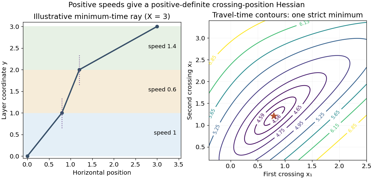
In each layer a minimum-time path is straight because the speed is constant there. The total time as a function of the two crossing positions isSetting its two partial derivatives to zero givesThe angles in the held diagram are measured from the vertical interface normals, so these ratios areThis is the layered-speed form of Fermat's principle and Snell's law. Signed horizontal displacements can be retained if the endpoint lies on the other side of the origin.

At a smooth interior stationary point, define $D=t_{11}{t}_{22}-t_{12}^2$. The second-derivative test gives a minimum for $D>0,t_{11}>0$, a maximum for $D>0,t_{11}<0$, and a saddle point for $D<0$; $D=0$ is inconclusive.

For the stated time function, putPositive physical speeds make all three coefficients positive. The positive Hessian of a layered travel-time functional here isThus the stationary path is a strict minimum, not merely a candidate of unspecified type. In fact the same positivity holds for all finite crossing positions, so the time function is strictly convex and the minimum is unique.

Take downward displacement as positive. At equilibrium, the lower spring carries $mg$ and extends by $mg/k$, while the upper spring supports both masses and extends by $2mg/k$. Write $x_1,x_2$ for the masses' downward displacements from these equilibrium positions. The extra upper-spring extension is $x_1$ and the extra lower-spring extension is $x_2-x_1$. Applying Newton's second law and cancelling the equilibrium forces givesThe gravitational terms disappear because the constant equilibrium spring forces already balance the weights. Gravity sets the equilibrium extensions, rather than the coefficients of the linear oscillation equations for ideal springs.

Set $\mathbf{x}=\mathbf{a}\cos (\omega t+\phi )$. The two normal modes satisfyThe characteristic equation is $(2-s)(1-s)-1=s^2-3s+1=0$. HenceHere $a_{\pm }$ denotes the scalar coefficient requested in the source, whereas bold $\mathbf{a}$ denotes a mode-amplitude vector. Both roots are positive.

For a mode with upper and lower displacement amplitudes $A,B$, the second equation gives $-A+(1-s)B=0$. ConsequentlyThese are signed ratios. The slow mode is in phase and the lower mass has the larger amplitude. The fast mode is out of phase and the upper mass has the larger amplitude. Taking an absolute ratio alone would discard the physically important relative phase.

Keep the same fixed laboratory equilibrium reference, and let the pivot move downward by $z(t)=z_0\cos {\omega }_{0}t$. The dynamic upper-spring extension is now $x_1-z$, soAt ${\omega }_0^2=k/m$, seek a particular solution ${\mathbf{x}}_p=\mathbf{b}\cos {\omega }_{0}t$. The amplitude equation isLet $s_{\pm }=(3\pm \sqrt{5})/2$, ${\omega }_{\pm }=\sqrt{k{s}_{\pm }/m}$ and ${\mathbf{u}}_{\pm }=(1-s_{\pm },1{)}^{\mathsf{T}}$. The unrestricted general motion isFour initial-condition constants are retained because none are specified. The driven particular response is not a resonance: ${\omega }_0$ differs from both eigenfrequencies. Its stationary upper mass is the pivot-driven two-mass spring antiresonance. Relative to the moving pivot, subtract $z(t)$ from both components.

The divergence theorem states ${\oint }_{\partial V}\mathbf{F}\cdot \hat{\mathbf{n}}dS={\int }_V\nabla \cdot \mathbf{F}dV$ with outward orientation. For $\mathbf{F}=(x,y,0)$, its divergence is $1+1=2$. The enclosed region has cylindrical bounds $0\le r\le 2$, $0\le z\le 4-r^2$, $0\le \varphi \le 2\pi$, so its volume isThereforeThe planar base contributes zero because its normal is vertical and $F_z=0$; the curved part accounts for the entire outward flux.

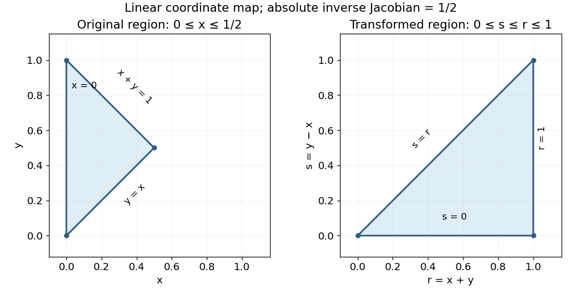
The original integration region is the triangle with vertices $(0,0)$, $(0,1)$ and $(1/2,1/2)$. Under $r=x+y$, $s=y-x$, its inverse map is $x=(r-s)/2$, $y=(r+s)/2$, with absolute inverse Jacobian determinant $1/2$. The boundaries $x=0$, $y=x$, $x+y=1$ become $s=r$, $s=0$, $r=1$. Thus the transformed triangle is $0\le s\le r\le 1$, andThe endpoint singularities are integrable after the inner integral: $r=0$ is only a collapsed vertex, while $r=1$ has the usual inverse-square-root behavior. The diagrams indicate the complete triangles, rather than rectangular bounds that would include points absent from the original region.

For an element $dx$, the vertical components of the approximately constant tension are $T{y}_x$ at its two ends. Their difference is $T{y}_{xx}dx$ to first order in the small slope. Its inertial response is $\rho dx{y}_{tt}$. Thus Newton's second law givesHere $\rho$ is mass per unit length. Small slopes, negligible gravity, uniform tension and negligible bending stiffness or dissipation are the assumptions in this wave equation on a string.

Use separation of variables, $y(x,t)=X(x)Q(t)$. The wave equation implies $X^{\prime \prime }/X=\ddot{Q}/(c^{2}Q)=-k^2$, giving $X^{\prime \prime }+k^{2}X=0$ and $\ddot{Q}+c^2{k}^{2}Q=0$. The fixed-end boundary conditions $X(0)=X(l)=0$ selectEach such product is a standing wave. A general released string is a superposition of these normal modes, not necessarily a single separated standing wave. Absence of damping keeps their amplitudes constant.

Use the product identity $\sin z\cos z=\frac{1}{2}\sin 2z$ to decompose the initial shape:The Fourier sine series is already explicit. Zero initial velocity gives cosine time factors, soand $y(x,t)=A\sin (\pi x/l)\cos (\pi ct/l)+(A/2)\sin (2\pi x/l)\cos (2\pi ct/l)$. Orthogonality of the sine modes makes this decomposition unique in the usual square-integrable fixed-end setting.

For one real mode $y_n=A_n\sin (k_{n}x)\cos ({\omega }_{n}t+{\varphi }_n)$, the kinetic and small-slope potential energy densities integrate toSince $\rho {\omega }_n^2=T{k}_n^2$, their sum is constant: $E_n=Tl{A}_n^2{k}_n^2/4$. The initial condition has ${\varphi }_n=0$ and $A_1=A$, $A_2=A/2$, henceAlthough the second mode's displacement amplitude is halved, its wavenumber and angular frequency are doubled, giving the same total energy. Orthogonality eliminates cross terms when the full string's energies are integrated.

The components of the curl of a gradient are differences of mixed second derivatives:If $\varphi$ has continuous second partial derivatives in a neighborhood, equality of mixed derivatives makes every component vanish. ThusThe $C^2$ condition is a sufficient regularity hypothesis; no simple-connectivity assumption is needed for this local identity. Topology matters for the converse assertion that every curl-free field has a global potential.

For the given polynomial vector field, direct differentiation givesAn exact differential is a differential one-form equal to $d\varphi ={\varphi }_{x}dx+{\varphi }_{y}dy+{\varphi }_{z}dz$ for a single-valued scalar function. This field is smooth on the simply connected domain ${\mathbb{R}}^3$, so its vanishing curl is sufficient for exactness. More concretely,The explicit potential proves exactness globally, rather than relying on curl-free behavior without checking the domain.

Integrate the first component of $\mathbf{F}=\nabla \varphi$ with respect to $x$:Matching the $y$ component gives $g_y=0$, and matching the $z$ component gives $g_z=0$. HenceThe fundamental theorem for line integrals now yieldsThe potential is a single-valued polynomial everywhere, so any piecewise smooth path with these endpoints has the same integral. The plus-gradient convention here should not be confused with the minus gradient of a mechanical potential energy.

Parametrize any actual particle trajectory by time, with $\mathbf{v}=\dot{\mathbf{r}}$ and acceleration $\mathbf{F}=\dot{\mathbf{v}}$. The chain rule givesIntegrating from the origin to the endpoint givesHere $K$ is specific kinetic energy, because the source defines it without a mass factor. Equivalently, $|{\mathbf{v}}_A{|}^2-|{\mathbf{v}}_O{|}^2=2$ in the chosen units. The individual initial or final speeds are not fixed by this result. For a particle of mass $m$, the change of ordinary kinetic energy would be $mI$.