Work with a nonsingular multivariate normal distribution, so is positive-definite. The claimed finite maximum-likelihood estimates also require the centered sample covariance matrix to be nonsingular; the exceptional case is discussed below.
Independence gives, up to a constant, the log-likelihoodLet and . The centered sum is zero, and expansion therefore givesFor every fixed positive-definite matrix , the extra quadratic term in the log-likelihood is , with unique maximum at .
Assume is positive-definite. Maximizing over now means minimizing . Put , another positive-definite matrix. ThenIf are its eigenvalues, the variable part is . The scalar inequality , with equality only at , shows that this is minimized uniquely at , or . ThusThe divisor is because this is maximum likelihood estimation, not the unbiased covariance estimate with divisor .
The nonsingularity condition matters. The centered scatter has rank at most . If is singular, choose , retain positive covariance eigenvalues on its range and let a covariance eigenvalue on its null space tend to zero. The quadratic likelihood term remains finite, while . This is singular covariance and nonexistence of a Gaussian maximum likelihood estimate: there is no finite maximizer over nonsingular . Under a nonsingular Gaussian population, is positive definite almost surely when ; for it is necessarily singular. The asserted estimate and the inverse in the next part have their usual meaning under .
By the spectral theorem, write , where is orthogonal and each . Choose the whitening transformationA linear image of a multivariate normal vector is multivariate normal, and . Thus are independent random vectors. Their whole joint distribution is independent of .
Define and . These satisfyThereforeThe right side is a function of independent standard multivariate normal observations only, so its distribution depends on but not on . This is the same affine invariance of Hotelling's statistic that permits multivariate mean tests with unknown covariance. The proof concerns the jointly transformed mean and covariance; whitening the mean alone would not establish the conclusion. Inverses exist almost surely under . If is singular, no square matrix can whiten it to , so nonsingularity of the population covariance is necessary as well.
The calculation is principal component analysis on a correlation matrix, rather than on an unscaled covariance matrix. For each of the eleven rating variables, subtract its column mean and divide by its column standard deviation. If is the resulting matrix, use the divisor convention of the fitted object to writeHere the scaling standard deviations use divisor , consistently with this convention. Using sample standard deviations with divisor gives the same correlation matrix and directions, with the corresponding score scale. Every diagonal entry of is one, so .
A principal component is the linear combination of the standardized ratings along . Its principal component score for judge is , and its variance is . The displayed component standard deviations are ; the explained variance of a principal component is . In particular,The first component explains about of the standardized variation, and the first two jointly explain . Components three, four and five add about , and . The cumulative line adds these proportions successively; it is not the proportion explained by that component alone. Retaining two components discards about of the total standardized squared variation.
The displayed principal component loadings are the unit eigenvector coefficients . The first direction has positive, broadly similar weights for all ratings. It measures an overall favorable-rating tendency: a judge high on most ratings has a high first score. The second direction compares integrity and demeanour, with large positive coefficients, against such attributes as decision promptness, case-flow management and physical ability, with negative coefficients. Thus among similarly rated judges, a positive second score indicates relatively stronger integrity/demeanour compared with those operational ratings. This is a description of a data direction, not a causal interpretation. Multiplying a whole eigenvector and its scores by minus one reflects the display but changes nothing substantive.
These principal component loadings are not themselves variable-component correlations. With standardized variables,For example, the integrity correlation with component one is approximately . Blank loadings in the printed second column indicate suppressed small entries, not exact zeros. The complete unrounded loading vectors in the fitted object must be used to calculate scores.
A two-dimensional representation plots the 43 pairswith each point labeled by its judge. In the fitted software object these are the first two columns of the score matrix. Nearby points have similar projections of their standardized ratings. The rank-two reconstruction is the orthogonal projection onto the leading principal plane and minimizes the total squared reconstruction error over all two-dimensional linear subspaces. To see this, for any orthonormal pair of directions the captured variance is the sum of its two Rayleigh quotients, at most by diagonalizing ; the remaining variance is the total minus that captured sum. Distances in the plot omit the smaller components, so a close projected pair need not be equally close in every original rating. The actual 43 coordinates cannot be recovered from the summary alone; the supplied data matrix or fitted score matrix is needed.
The printed descriptive list omits INTG, although the loading table includes it. INTG denotes integrity and supplies the eleventh variable. The standard data set also contains a contacts variable; the stated eleven-rating analysis uses the ratings, not contacts.
The response is the species categorical variable, while the four measurements are candidate predictors. The dot in the formula means all other columns of the data frame. The fitted object is a classification tree: it recursively partitions predictor space by binary threshold rules and assigns a species and class-probability vector to each terminal region. Sepal width was available but was not selected in the displayed tree.
At a node , let be the number of observations of class and . The multinomial likelihood is maximized by . The fitted class is one attaining the largest proportion, with a software convention resolving ties. The classification-tree deviance isA pure node has zero deviance. At each nonterminal node, consider candidate split points between distinct observed predictor values, and choose the split with the largest decrease . Repeating this local maximization constructs a binary decision tree; it does not solve a global optimization over all trees. Growth stops when nodes are pure or size/deviance controls prohibit further splitting. Mixed leaves with five or six observations can therefore remain. The node number has children and , and a terminal-node marker means that no further split was retained.
The probability triples are in class order , not . For example, the pure left leaf has probability vector and predicts , while the 54-observation node has counts and predicts . The root counts are , giving and a tied majority class. Its reported choice of does not indicate a more common class.
The complete derived decision rule is shown below. Each leaf includes its fitted class and the observed class counts, so both the branching logic and its remaining errors are visible. For the observed data, the printed strict inequalities leave no equality cases because the thresholds fall between measurement values. A consistent right-branch convention at equality extends the rule to new specimens.
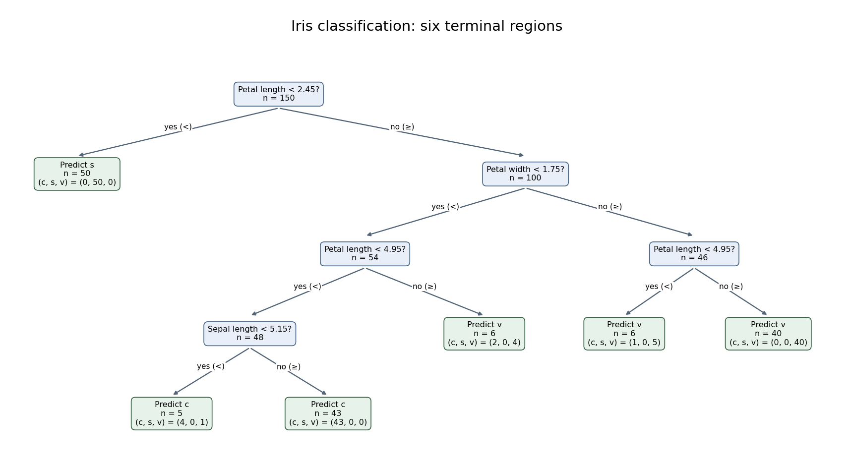
Six-leaf iris classification tree with fitted classes and class counts at every terminal node
. Details. 
The six terminal nodes contain the class countsThus the training misclassification error isThe terminal classification-tree deviance is insteadThe displayed residual mean deviance divides this by , yielding approximately . This is the summary's reporting convention, not a normal-error residual mean square or an automatic chi-squared calibration with 144 statistical degrees of freedom. The two summary measures answer different questions: deviance depends on the fitted probability of each observed class, while misclassification counts only whether the majority-class prediction is correct. Both are training quantities. Cross-validation or independent test data, rather than the displayed training error, are needed to assess prediction on new specimens; cost-complexity tree pruning can select a less elaborate tree if predictive performance warrants it.
A randomized complete block design groups similar experimental units into experimental blocks and places every treatment once in each experimental block, independently randomizing treatment allocation within experimental blocks. Blocking removes background between-block variation from within-block treatment comparisons. A balanced incomplete block design has treatments and experimental blocks of size , with each treatment occurring in experimental blocks and every distinct treatment pair together in experimental blocks. Counting treatment occurrences and co-occurrences gives and .
A Latin square of order places each of treatment symbols once in every row and every column of a array. This controls two nuisance directions. A Graeco-Latin square superposes two mutually orthogonal Latin squares: each square is Latin, and each ordered pair of symbols from the two squares occurs exactly once. The two symbol factors can then be fitted together with row and column effects. Random permutations of row labels, column labels and treatment symbols provide a suitable randomized allocation without destroying these balances.
For the operator experiment, fit the additive normal linear modelHere account for the two fabric directions, and is the operator effect. Additivity, independent equal-variance errors and the normal assumption supply the exact F-test; there is only one observation per cell, so an unrestricted interaction model is not available.
In the analysis of variance for a Latin square, the three centered factor spaces each have dimension . Together with the intercept the model has rank ten, leaving residual statistical degrees of freedom. The corrected total has . The completed calculation isUnder the null hypothesis , the operator F-statistic isThe upper five-percent critical value for is , so the operator effect is not significant at five percent in this model.
The decision is independent of the order of fitting rows, columns and operators. To prove the required orthogonality, let be any centered row coefficients and any centered operator coefficients. Their observation-space inner product is , since every operator occurs once in each row. The same calculation applies to columns and operators, and all row-column pairs occur once as well. Thus the three centered spaces are mutually orthogonal; their projections commute and sequential sums of squares equal adjusted sums of squares in every fitting order.
With machines included, the layout is a Graeco-Latin square: the machine symbols are Latin, and all sixteen operator-machine pairs occur exactly once. Fitin addition to the earlier constraints. The machine space contributes three new statistical degrees of freedom and is orthogonal to the previous factor spaces, so the operator sum of squares remains . The residual sum of squares and statistical degrees of freedom becomeHenceThis exceeds but not . Therefore the operator effect is now significant at five percent, but not at one percent. Adjustment for machines has removed substantial residual variation without altering the operator numerator. This illustrates why a balanced nuisance factor can change precision and significance even when it does not change the estimated treatment contrasts.
Code each factor level by . A nonconstant factorial contrast indexed by a nonempty factor set has sign column . Flipping any coordinate in reverses that sign and pairs the treatment combinations, so exactly have each sign. Allocating the two signs to two experimental blocks therefore divides the full factorial design into equal experimental blocks. The contrast is confounded with experimental blocks because its column is constant within each experimental block: changing its coefficient and compensating by the two experimental block intercepts leaves every fitted value unchanged. It has no information separate from experimental block differences. Randomize the allocation of the two groups to days and the run order within days.
Write for temperature, pressure and catalyst, respectively, with low levels and catalyst one coded minus. In the supplied allocation, on day one and on day two. Thus the three-factor interaction is confounded with days. Every other nonconstant factorial column is orthogonal to the day contrast, because its product with is a nonconstant sign column on the full cube and consequently sums to zero.
If all interactions are negligible, the fitted model contains an intercept, one day contrast and the three main effects. The corrected total statistical degrees of freedom partition asThe three residual statistical degrees of freedom are the unused two-factor interaction columns , pooled as error under the stated negligible-interaction assumption. There is no independent pure-error replication of treatment combinations.
For four days with two runs each, all three main effects can be estimated. One regular allocation pairs each treatment combination with its complete opposite:The block-generating columns can be and ; their product is also constant in experimental blocks. Thus span the three experimental block contrasts, while and vary within experimental blocks. The main effects remain mutually orthogonal and separate from the experimental block effects; with an additive main-effect model there is one residual degree of freedom, represented by .
For the further request about , the distinction between regular confounding and unrestricted pairing is important. A regular four-block allocation cannot retain all three main effects and . Its three confounded columns form a rank-two defining subgroup. To preserve main effects, these columns must lie in . If the subgroup includes and a two-factor column, their product is a main-effect column, which is forbidden. Hence the only permissible nonidentity subgroup is , and it necessarily confounds . This proves impossibility in the usual regular factorial-blocking framework, rather than relying on a count of available statistical degrees of freedom.
The literal request does not explicitly restrict arrangements to regular experimental blocks. If arbitrary pairings are permitted, a nonregular construction can estimate together, assuming the other interactions are omitted from the model. An explicit allocation isEvery treatment combination occurs exactly once. Fit one unrestricted intercept per day and the four coefficients . By estimability from within-block differences, subtracting the second run from the first in each experimental block removes all day effects and yields the coefficient matrixThus all four coefficients are uniquely determined from the four day differences. In this broader design class the answer is yes, under the reduced four-effect model. The resulting fit is saturated: four experimental block intercepts plus four treatment coefficients use all eight observations, leaving no residual estimate of error variance. Replication or external error information would be needed for inference. This does not contradict the impossibility for regular orthogonal confounding, and it does not claim simultaneous unbiased estimation when arbitrary additional interactions are retained.
Let and let an approximate experimental design specify the proportions of observations allocated to points of the design region. Its normalized information matrix of an experimental design isFor independent equal-variance observations realizing those proportions, , and the least-squares estimator has covariance matrix . A D-optimal design maximizes , equivalently minimizing the determinant of this covariance at fixed . A G-optimal design minimizes the largest variance of a fitted regression mean over the design region, equivalentlywhere is the design sensitivity function. This is the variance of the estimated mean multiplied by , not the variance of a new noisy observation.
For continuous regressors spanning a -dimensional parameter space on a compact design region, the general equivalence theorem for optimal design states that, among approximate designs with nonsingular information matrices, the following are equivalent: being a D-optimal design, being a G-optimal design, andAt every support point of an optimal design, . To see the criterion, the sensitivity average is , so the supremum is at least . Adding an infinitesimal allocation at has directional derivative for . At a D-optimum each derivative is nonpositive. Conversely, if all sensitivities are at most , the tangent bound for the concave function shows that no competing design increases it. A nonsingular D-optimum exists by the spanning assumption and compactness of the information-matrix set, so the smallest possible G-value is also . Equality at support points follows from the average. The theorem refers to the full approximate-design class; constrained integer allocations or mandated augmentations require separate comparison.
For the linear mean , take . Equal replication at the four corners givesAll odd corner sums and the sum of vanish, while each squared regressor sum is . If is the mean of the observations at , , the least-squares normal equations giveIn particular the intercept is the average of the four cell means, and each slope is the average of its sign-weighted cell means. Independence and equal error variance suffice for this covariance formula; normal errors are not needed for it.
The normalized corner design has , so its sensitivity iswith equality at all four corners. Since , the general equivalence theorem for optimal design proves that the equally weighted corner design is D-optimal and G-optimal.
For the augmentation, all added observations share the regressor . The enlarged design matrix satisfiesBy the matrix determinant lemma,For the permitted nine points, the determinant is at the center, at an edge midpoint and at a corner. ThereforeAll four corners tie for the best mandated single-point augmentation. This is optimality among the specified augmented designs, not unrestricted D-optimality with observations: the resulting normalized determinant is , whereas equal corner proportions have determinant one. The restriction that the extra runs all occur at one point is what prevents recovering equal proportions.
Articles by others on the same topic
There are currently no matching articles.