Past exam of the mathematics course of the University of Cambridge / 2007 / ia / Paper 2

The differential operator is $(D-3{)}^2$, where $D=d/dx$. Factoring out the forcing's exponential removes this repeated characteristic root of a constant-coefficient differential equation: set $y=e^{3x}v$. Differentiation gives $(D-3)y=e^{3x}{v}^{\prime }$ and $(D-3{)}^{2}y=e^{3x}{v}^{\prime \prime }$, so $v^{\prime \prime }=\cos (2x)$. Two integrations yieldThe initial conditions become $v(0)=0$ and $v^{\prime }(0)+3v(0)=1$, hence $B=1/4$ and $A=1$. ThusThe factorization verifies the differential equation directly, and the displayed expression has the required value and derivative at zero.

Put $F(y)=(y^2-4)\arctan y$. Its zeros, and hence the equilibrium points, are $-2,0,2$. For a perturbation $y=y_{\ast }+\eta$, linear stability analysis gives $\dot{\eta }=F^{\prime }(y_{\ast })\eta +O({\eta }^2)$, withAt zero, $F^{\prime }(0)=-4$, so sufficiently small perturbations decay and $y=0$ is asymptotically stable. At either outer equilibrium point, $F^{\prime }(\pm 2)=4\arctan 2>0$, so $y=-2$ and $y=2$ are unstable. The phase line confirms the result: $F$ has signs $-,+,-,+$ on the intervals cut out by $-2,0,2$, respectively. Flow points toward zero on both sides and away from both outer equilibria.

The constant solutions are fixed points of $G(u)=u^2(1+u)/2$. Solving $G(u)=u$ gives $u(u+2)(u-1)=0$, hence $u_{\ast }=0,-2,1$. For a discrete dynamical system, a small perturbation satisfies ${\eta }_{n+1}=G^{\prime }(u_{\ast }){\eta }_n+O({\eta }_n^2)$, whereA multiplier of magnitude less than one contracts perturbations; a multiplier greater than one expands them. Therefore $u=0$ is asymptotically stable, while $u=-2$ and $u=1$ are unstable. In particular, if $|u|\le 1/2$, then $|G(u)|\le (3/4)|u{|}^2\le (3/8)|u|$, proving convergence to zero without relying solely on the vanishing linear multiplier.

For $0\le u\le 1$, independence givesThus $U$ has probability density function $f_U(u)=2(1-u)$, and its expected value isPointwise, $U+V=X+Y$ and $UV=XY$. By linearity of expectation, $\mathbb{E}V=1-1/3=2/3$; by independence, $\mathbb{E}(UV)=\mathbb{E}X\mathbb{E}Y=1/4$. Consequently the covariance of two uniform order statistics isThe order statistics are dependent despite the independence of the original observations.

The moment-generating function of a random variable $X$ is $M_X(t)=\mathbb{E}(e^{tX})$, defined for real $t$ where that expectation is finite. For a standard normal distribution, completing the square givesIt is finite for every real $t$. Derivatives at zero give the moments: the expansion $e^{t^2/2}=1+t^2/2+t^4/8+O(t^6)$ therefore givesFor $Y$ with the normal distribution of mean $\mu$ and variance ${\sigma }^2$, write $Y=\mu +\sigma X$ in distribution. Its moment-generating function is consequentlyThis formula also covers the constant random variable when $\sigma =0$.

In the normalized second-order linear differential equation, an ordinary point $z_0$ is one at which both $p$ and $q$ are holomorphic functions in a neighbourhood of $z_0$. A singular point of a differential equation is a point that is not ordinary. A singular point $z_0$ is a regular singular point if $(z-z_0)p(z)$ and $(z-z_0{)}^{2}q(z)$ extend analytically to $z_0$. Equivalently, $p$ has at most a simple pole and $q$ at most a double pole there. If a singular point fails this test, it is an irregular singular point. The normalized form matters: zeros of a leading coefficient must first be assessed after division by that coefficient.

For $z\ne 0$, division by $4z$ gives $p(z)=1/(2z)$ and $q(z)=1/(4z)$. Thus zero is singular, but $zp=1/2$ and $z^{2}q=z/4$ are analytic. Zero is a regular singular point.

Apply the Frobenius method with $y=z^r{\sum }_{n=0}^{\infty }{a}_n{z}^n$, $a_0\ne 0$. The lowest power $z^{r-1}$ has coefficient $[4r(r-1)+2r]a_0$, so the indicial equation is $2r(2r-1)=0$. Its characteristic exponents at a regular singular point are $0$ and $1/2$. At the next powers,With $a_0=1$, the two Frobenius solutions are thereforeBoth analytic power-series factors converge everywhere by the ratio test. Recognizing the trigonometric series givesOn a punctured neighbourhood choose a consistent square-root branch for the second solution; the first is entire in $z$. These solutions are independent, since their leading orders are $1$ and $z^{1/2}$. A direct square-root reduction of a regular-singular differential equation also verifies the closed forms: for $s=\sqrt{z}$ and $Y(s)=y(s^2)$, $4z{y}^{\prime \prime }=Y_{ss}-Y_s/s$ and $2y^{\prime }=Y_s/s$, so the equation reduces to $Y_{ss}+Y=0$.

Write $u(x,y)=U(\xi ,\eta )$. The chain rule gives ${\partial }_x={\partial }_{\xi }+{\partial }_{\eta }$ and ${\partial }_y=2{\partial }_{\xi }+3{\partial }_{\eta }$. Consequently the coefficients of $U_{\xi \xi }$ and $U_{\eta \eta }$ cancel, while that of $U_{\xi \eta }$ is $12-25+12=-1$. The transformed partial differential equation is $-U_{\xi \eta }=1$. Integrating once in each variable gives the most general twice differentiable solution,where $F,G$ are arbitrary twice differentiable functions. The change of variables is invertible because its Jacobian determinant is $3-2=1$.

On $y=0$, the value condition gives $F(x)+G(x)=x^2$. Differentiating it yields $F^{\prime }(x)+G^{\prime }(x)=2x$. The derivative condition gives $-5x+2F^{\prime }(x)+3G^{\prime }(x)=x$. Subtraction therefore gives $G^{\prime }(x)=2x$ and $F^{\prime }(x)=0$. The constants in $F$ and $G$ cancel in their sum, leavingIndeed $u_{xx}=0$, $u_{xy}=1$, $u_{yy}=6$, so the original operator gives $-5+6=1$, and the two initial-line conditions hold.

Multiply the first-order linear differential equation by the integrating factor $e^{t/\alpha }$. ThenIf $y\to 0$ in the remote past, then $e^{t/\alpha }y\to 0$ there. Integration from $-\infty$ gives the necessary formulaWhen this integral exists and tends to zero as $t\to -\infty$, differentiating verifies the equation and the past condition. Two such solutions differ by $C{e}^{-t/\alpha }$, which diverges at $-\infty$ unless $C=0$, proving uniqueness. This is the causal response of a first-order relaxation equation, a convolution with its decaying impulse response.

The phrase “general function” implicitly requires compatibility with the past condition: it does not guarantee existence for arbitrary $f$. A sufficient condition is bounded forcing with $f(t)\to 0$ as $t\to -\infty$; after setting $r=t-s$, the integral is bounded by the supremum of $|f|$ before $t$. For example, $f\equiv 1$ gives $y=1+C{e}^{-t/\alpha }$, so no solution has the stated past limit. Both forcings below vanish in the past and meet the intended causal condition, the impulse being interpreted distributionally.

Inserting the Dirac delta forcing into the integral gives the impulse responseIt is zero before the impulse and obeys the homogeneous equation afterward. Integrating the equation across zero gives $\alpha [y(0^{+})-y(0^{-})]=1$, exactly the jump $1/\alpha$ in this formula. Thus the formula also verifies the differential equation as a distribution; assigning a particular value at the jump does not affect that distribution.

For the Heaviside step function forcing, the integral begins at zero when $t>0$:Before zero it vanishes. ThereforeThis causal response of a first-order relaxation equation is continuous at zero and approaches the new constant equilibrium exponentially.

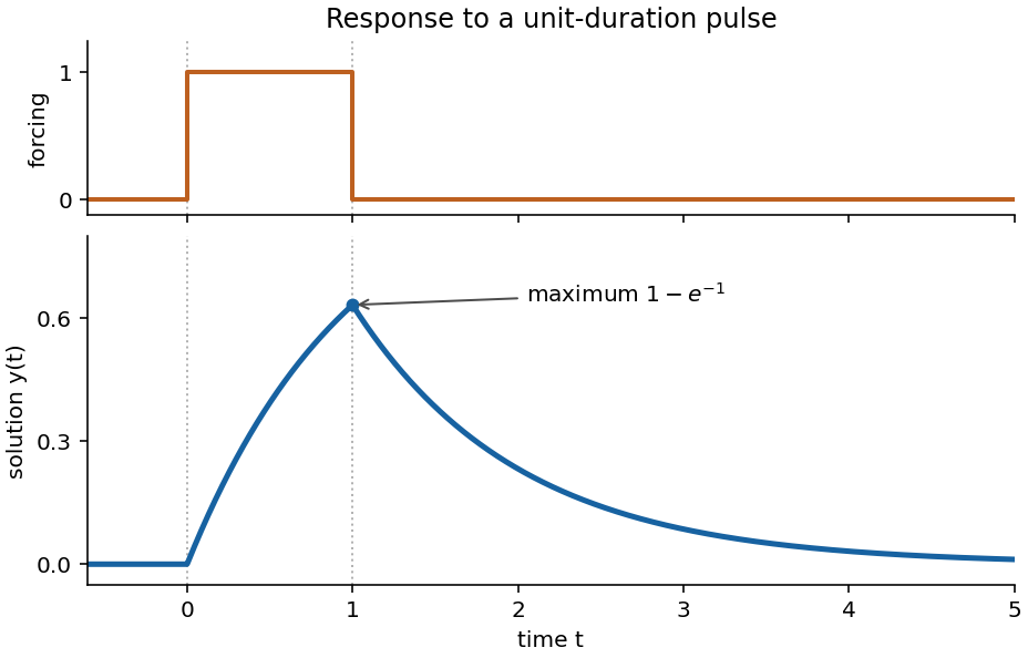
The forcing is a unit pulse on $0<t<1$. For $t<0$, the homogeneous equation and continuity with $y(0)=0$ give $y=0$. On $0<t<1$, integration with $y(0)=0$ gives $y=1-e^{-t}$. At the end of the pulse its value is $1-e^{-1}$, and the subsequent homogeneous decay must start at that value. ThusEquivalently it is the difference of two translated step responses, $(1-e^{-t})H(t)-(1-e^{-(t-1)})H(t-1)$. The solution is continuous, rises concavely to its maximum $1-e^{-1}$ at $t=1$, and then decays exponentially to zero. Its derivative has jumps at the pulse edges; those are permitted because the right-hand side has step discontinuities.

For the homogeneous linear recurrence relation, a trial $u_k=r^k$ gives the characteristic equation of a linear recurrence $r^2+5r+6=(r+2)(r+3)=0$. Thus the two homogeneous sequences are $(-2{)}^k$ and $(-3{)}^k$. Seek a particular solution $u_k=ak+b$; substitution gives $12ak+12b-5a=12k+1$, so $a=1$ and $b=1/2$. HenceThe two independent constants supply arbitrary initial values for this second-order linear recurrence relation.

The homogeneous sequences are again $(-2{)}^k$ and $(-3{)}^k$. A particular solution $D{2}^k$ has left-hand side $10D{2}^k$, so $D=1/10$. Consequently $y_k=A(-2{)}^k+B(-3{)}^k+2^k/10$. The two initial conditions require $A+B=9/10$ and $-2A-3B=4/5$, giving $A=7/2$ and $B=-13/5$. ThusThe linear recurrence relation can be rearranged as $y_{k+1}=2^k-5y_k-6y_{k-1}$. Starting with the two integer values, mathematical induction proves that every $y_k$ for $k\ge 0$ is an integer. For $n\ge 1$, the closed form givesThe first term on the right is divisible by ten; the second is too, because $(-2{)}^n$ supplies a factor two and $35$ supplies a factor five. Therefore $10$ divides $2^n-26(-3{)}^n$ for every positive integer $n$. The positivity condition matters: at $n=0$ the expression is $-25$.

For a nonnegative integer-valued random variable, its expected value is $\mathbb{E}N={\sum }_{r=0}^{\infty }r{p}_r$, allowing the value $+\infty$. Since $r={\sum }_{n=1}^{r}1$, rearranging nonnegative summands gives the tail-sum formula for expectation:No integrability assumption is needed for the rearrangement. The same formula holds for an extended nonnegative integer-valued variable by the monotone convergence theorem, using $N={\sum }_{n\ge 1}{1}_{\{N\ge n\}}$.

For the first ascent in independent continuous observations, continuity makes ties probability zero. By order symmetry of independent random variables, the first $m$ observations have each of their $m!$ strict orderings with equal probability. For $n\ge 2$, $N\ge n$ means exactly that the first $n-1$ observations are decreasing, soSubtracting consecutive tails giveswith probability zero for $r=0,1$. The events $\{N\ge n\}$ decrease to $\{N=\infty \}$; continuity of probability under decreasing intersections gives $P(N=\infty )={\lim }_{n}1/(n-1)!=0$. Finally,The first observation cannot itself end the run; this is why the tail includes the separate term $P(N\ge 1)=1$.

The inverse change of variables is $x=u$, $y=(v-u)/a$, with absolute Jacobian determinant $1/a$. Because the original random variables are independent, their joint density is $f(x)g(y)$. Thus the transformed joint density isThe support is important: $X,Y\ge 0$ implies $V\ge U\ge 0$.

For independent exponential random variables of rate $\lambda >0$ and $a=1/2$, this becomes $2{\lambda }^2{e}^{-2\lambda v+\lambda u}$ on $0\le u\le v$. Integrating out $u$ gives the density of the sum:It vanishes for $v<0$. On the other hand, the cumulative distribution function of the maximum isDifferentiating yields exactly the same density. The maximum and $X+Y/2$ have the same distribution, as described by maximum of two exponentials as a scaled sum; this does not assert that they are equal for the same pair of sampled values.

The statement is true. Put $C_k={\bigcap }_{r=1}^k{A}_r$. The assumed $P(C_{n-1})>0$ ensures that every conditioning event $C_{k-1}$, $2\le k\le n$, has positive probability. By the definition of conditional probability,Multiplying makes the fractions telescope, givingThis proves the chain rule for probabilities here without any assumption of independence. The final numerator $P(C_n)$ may be zero; all denominators remain positive.

The statement is true. Use the union bound on the complementary events:This proves the claim for arbitrary events, with no independence requirement.

The statement is true. For $n\ge 2$, being in every pairwise intersection is equivalent to being in all the events:Indeed every index occurs in at least one pair. Apply the union bound to the complements of these $\left(\genfrac{}{}{0ex}{}{n}{2}\right)$ pairwise intersections to obtainThis is positive common intersection from pair-intersection probabilities. It remains valid for $n=2$, where it reduces to the asserted positivity of the single pairwise intersection.

The statement is false. Take two independent fair bits $U,V$ on the four equally probable outcomes $00,01,10,11$, and put $A_1=\{U=0\}$, $A_2=\{V=0\}$, and $B=\{U=V\}$. Each of $A_1,A_2,B$ has probability $1/2$, andThus $B$ is independent of each event separately. But $A_1\cup A_2$ contains $00,01,10$, whereas its intersection with $B$ contains only $00$. ThereforeThis is a concrete failure of extending separate independence to the generated union. A counterexample at the permitted value $n=2$ disproves the universal claim; for any larger $n$ one can repeat $A_1$ as the additional events.

Let $\Theta =\angle AOB$ and let the sphere have radius $R$. By rotational invariance, condition on $A$ and place it at the north pole. A band at polar angle $\theta$ has surface area $2\pi R^2\sin \theta d\theta$, while the sphere has area $4\pi R^2$. Thus the central angle between independent uniform sphere points has densitywith density zero outside that interval.

Condition now on $A,B$ with their angle fixed at $\theta$. For $\angle AOC$ and $\angle BOC$ to be acute, the unit position vector of $C$ must have positive dot products with both unit vectors of $A$ and $B$. Hence $C$ must lie in the intersection of the two corresponding open hemispheres. The great circles bounding them meet at the two antipodes perpendicular to the plane of $A,B$. Their common hemisphere region is a spherical lune of opening $\pi -\theta$: when $A=B$ it is a hemisphere of opening $\pi$, and as the two normals separate, that opening decreases by $\theta$. More explicitly, take the common boundary antipodes as poles. The longitude conditions each allow an interval of length $\pi$, with their centres separated by $\theta$, so the intersection has longitude width $\pi -\theta$.

Integrating the spherical area element $R^2\sin \phi d\phi d\lambda$ over that lune gives area $2R^2(\pi -\theta )$. Thus the conditional probability that the two angles involving $C$ are acute is $(\pi -\theta )/(2\pi )$. The remaining angle $\Theta$ must itself be acute, so the desired probability isIntegration by parts gives ${\int }_0^{\pi /2}\theta \sin \theta d\theta =1$, while ${\int }_0^{\pi /2}\sin \theta d\theta =1$. ThereforeThis calculates pairwise acute central angles of three uniform sphere points by conditional area, rather than incorrectly treating the three angle events as independent. Boundary right angles have probability zero, so choosing open rather than closed hemispheres does not change the result.