The three spherical basis vectors form an orthonormal basis: their displayed Cartesian components have unit lengths and pairwise zero dot products. For an orthonormal basis, a vector is the sum of its projections onto the basis vectors. Taking the dot product of each Cartesian unit vector with each spherical unit vector therefore gives the inverse change of basis:Equivalently, the change-of-basis matrix is orthogonal, so its matrix inverse is its transpose. These formulas use the stated angular convention for spherical polar coordinates; at a pole the tangential basis vectors still depend on the chosen azimuth.
Use suffix notation, summing repeated indices, and the Levi-Civita symbol convention . Contracting the outer symbol with the symbol from the second cross product gives the epsilon-delta identitywhere is the Kronecker delta. ThusThe second term is zero because is symmetric in and the Levi-Civita symbol is antisymmetric. The cyclic rearrangement of the remaining symbol has positive sign. Its contraction is the scalar triple product . HenceThis cross products with a common vector identity requires no independence assumption, so it also covers zero or parallel vectors.
The coefficient matrix has determinantA square linear system has a unique solution for every right-hand side precisely when its coefficient matrix is an invertible matrix. Here a unique solution exists exactly when , for every real .
For an explicit Gaussian elimination, subtract twice the second equation from the third, then use the second equation, obtaining and . The first equation determinesand the preceding formulas determine . When this last coefficient vanishes; the next parts determine compatibility rather than dividing by zero.
For , the third coefficient row equals three times the second minus twice the first. The first two rows are independent, so the coefficient matrix rank is two. The same dependence must hold for the right-hand side, givingThus infinitely many solutions occur exactly for and . The null space has dimension one by the rank-nullity theorem, and an explicit parameterization, with , isSubstitution verifies all three equations in each family.
When but , the dependent coefficient rows would require an impossible equality between their right-hand sides. Thus the augmented matrix has larger matrix rank than the coefficient matrix, and the linear system is inconsistent. For part (i) already supplies a unique solution. Consequently there is no solution exactly when and .
The two-variable arithmetic-geometric mean inequality follows from a square:Hence , with equality exactly when .
For the series, apply that same inequality with and to obtainThe comparison series converges: its first summand has finite sum by hypothesis, and the inverse-square series converges, for example by the telescoping estimate for . Thus the comparison test for series provesEquivalently, its positive partial sums are increasing and bounded above by , so the bounded monotone sequence theorem proves convergence directly. This is the case of weighted square roots of a summable sequence.
First establish a comparison fact for a power series. If it converges at , its terms are bounded, say . For ,by the geometric series. Thus convergence at one point implies absolute convergence at every point of smaller modulus.
Let be the set of moduli of points at which the power series converges. It contains zero. Define the radius of convergence . If , the definition of supremum gives a convergent point with ; the comparison just proved gives absolute convergence at . This reasoning also applies when . If and the power series converged there, its modulus would belong to , contradicting the definition of . ThereforeThe boundary is intentionally undecided by this argument. If , only the exterior assertion is nonvacuous.
For the particular coefficients for , comparison with gives absolute convergence whenever . If , then fails to tend to zero: its successive ratio is , eventually greater than a fixed number bigger than one. The necessary term condition for convergence of a series therefore fails. HenceFor instance the positive boundary point gives the divergent harmonic series; no assertion of universal boundary convergence is needed.
Decompose the position vector into its components parallel and perpendicular to the unit vector :This is an orthogonal projection, and the Pythagorean theorem gives . The two surfaces are distinguished by fixing an angle in part (a), and fixing distance from an axis in part (b).
For , the dot product equation says that the angle between and the oriented unit vector satisfies . Thus is fixed. More explicitly, using the orthogonal projection from the introductory solution,Consequently the surface is one infinite nappe of a right circular cone, with apex at the origin, including the apex itself. The cone's axis points along , and its acute semi-angle is . Equivalently, is the cosine of the angle from the oriented axis. Squaring the original equation without retaining the sign of would incorrectly add the opposite nappe of a double circular cone. No base disk is included in this infinite lateral surface.
The vector is the perpendicular component of relative to the axis , so its length is the distance from that axis. Hence the surface is an infinite circular cylinder of radius about the line through the origin parallel to . Here is the radius and fixes the axis direction; reversing leaves the same circular cylinder.
If are an orthonormal basis of the plane perpendicular to , a parameterization isThis verifies that all heights and all angular positions, but no interior points, belong to the surface.
The sphere-plane intersection is governed by the orthogonal projection of the sphere's centre onto the plane. Since has unit length, let , the signed distance from to the plane along . The following parts determine the centre and radius and retain this sign; the radii alone cannot distinguish the two possible sides of the oriented plane.
Set , where . Then , so lies in the plane. For any position in that plane, is perpendicular to . The Pythagorean theorem therefore givesOn the sphere the left side is . Thus the intersection is the circle in the plane centred at , with squared radius . Its centre must therefore be , andIn terms of the radii, , with the sign fixed by . In the central-plane case , both signs give zero. This is the center and radius of a sphere-plane intersection formula with its orientation made explicit.
Substitute the signed displacement into the Pythagorean theorem relation from part (a):A genuine circle requires . Equality gives a tangent plane and a single point, interpreted as radius zero; a larger distance gives no intersection. Under the stipulated circle intersection, the radicand is positive. Its centre is .
Write , with . The linear map sends to and sends to . On the perpendicular plane, and are perpendicular vectors of equal length. ThusThe expression in parentheses is a rotation in three dimensions by about the oriented axis, with the positive direction fixed by the cross product. Therefore the map scales the axial component by , scales the perpendicular component by , and rotates the perpendicular plane by . Since , the angle lies between zero and . This is an axis-angle decomposition, with different axial and transverse scale factors.
In suffix notation, , so the matrix entries areHere is the Kronecker delta and the Levi-Civita symbol. The diagonal determines . Comparing the off-diagonal entries withgives . As is a unit vector and , and . ThusIn this example the transverse scaling is and the axial scaling is two; the rotation angle is .
Let be the axial orthogonal projection and . Then , while the vector triple-product identity gives . The map is . Its inverse is on the axis. On the perpendicular plane,Thus the inverse of an axis-angle linear map isor, in the requested vector form,The denominators are nonzero because . Multiplication on each invariant component verifies the matrix inverse without choosing a coordinate frame.
For the Cauchy-Schwarz inequality, take and use positivity of the inner product:Multiplication by provesEquality holds exactly when . Positive definiteness of the inner product makes this equivalent to . Conversely, substitution of a scalar multiple gives equality. Thus equality holds precisely for linearly dependent nonzero vectors.
Apply the Cauchy-Schwarz inequality to and in the Euclidean inner product on . It givesAfter expansion and division by two,The equality criterion from the introductory proof says . One can also see both the inequality and equality case from .
Set and . The expression in the equation is . Apply the Cauchy-Schwarz inequality in toTheir dot product is , and . Thus the expression is nonnegative, and it is zero precisely when equality holds in Cauchy-Schwarz. That requires . The fourth coordinate forces , and the other three coordinates then giveSubstitution gives , so this unique possible choice really is a solution.
Write a straight line in Cartesian form , where are real and . With , set and . Using the complex conjugate,Thus the real linear equation of a line in the complex plane isConversely, writing gives , an ordinary straight line with normal vector . The nonzero condition on matters: would give either the whole complex plane or the empty set.
The quotient is defined only when . Its unit-modulus condition then gives . On expanding with complex conjugates,Hence at least one imaginary part is zero, and either or is real. Conversely, either reality condition makes the two squared moduli equal; provided the denominator is nonzero, the quotient has modulus one. No conclusion is drawn from an undefined quotient.
For real at which the denominator is nonzero, mapping to the unit circle gives . There are infinitely many such real , so the resulting quadratic polynomial identity has all coefficients zero:If , the first equality gives , contradicting the nonzero determinant . Thus . Put , and . The equalities becomeTwo complex numbers with equal real parts and equal moduli have imaginary parts equal in magnitude. Consequently or . The first option would give , so it is excluded. The second givesMoreover must be nonreal, since otherwise the two options coincide and the map would be constant. This proves the Möbius transformations from the real axis to the unit circle representation directly from coefficients.
Conversely, for real , the numbers and are complex conjugates, and their moduli agree. Nonreal ensures the denominator is nonzero on the real line; multiplication by preserves modulus. At the point at infinity on the Riemann sphere, the map takes the value . Thus the representation also respects the extended real axis.
Let for . This is an increasing continuous function. Starting at , induction gives : if , then , and every iterate is at least .
The first step has . Since is increasing, implies . Thus this sequence is increasing and bounded above. Let . For every , a term exceeds ; all later terms lie between it and . This proves convergence, the elementary bounded monotone sequence theorem.
For the second starting value, write the iterates as and . Here . Monotonicity of propagates this inequality, so is decreasing. It is bounded below by because every positive iterate is at least that value. Hence it converges to its infimum . From onward all terms lie in .
Continuity of permits passing to each limit in the recurrence, giving . To prove that these fixed points agree, suppose both satisfy that equality. Subtracting the two equations and rationalizing givesThe second factor is positive: , whereas . Thus . ThereforeExistence has been supplied by the two convergent sequences, and the subtraction argument gives the required uniqueness in their common interval.
The mean value theorem states that a real-valued function continuous on and differentiable on , with , has a point such thatFor the proof, subtract the secant line and put . Then . If is identically zero, every interior point works. Otherwise it has a positive maximum or a negative minimum. The extreme value theorem supplies that extremum, and its nonzero value makes its location interior. At an interior differentiable extremum, the difference quotients on the two sides have opposite weak signs, so their common limit is zero. Hence , proving the formula. This also gives the Rolle theorem argument rather than merely citing it.
Because exists everywhere, is differentiable everywhere and therefore continuous everywhere; continuity of is not required. For , apply the mean value theorem to on . It gives withFor equality is immediate. Hence is nondecreasing: implies .
Put . Since and , . Apply the mean value theorem separately to and . There exist and such thatThese are the requested points, and . Part (i) makes , so the corresponding secant slopes satisfyMultiply by the positive denominators and collect to obtainThis is precisely the defining chord inequality for a convex function. The proof uses only existence and nonnegativity of , with no additional regularity hypothesis on that derivative.
To prove boundedness on , suppose instead that is unbounded and choose with . The Bolzano-Weierstrass theorem gives a subsequence converging to . Continuity then gives , contradicting . Hence is bounded.
Let and . Choose with . Another application of Bolzano-Weierstrass theorem yields a subsequence tending to , and continuity gives . Applying the same argument to gives with . ThusThis proves the extreme value theorem here, including both attainment assertions.
For , its two limits supply such that whenever . On , continuity and the result just proved give a finite bound . Consequently on the whole real line.
For the final value assertion, if , take . Otherwise . The positive-infinity limit gives a point with , so . The intermediate value theorem on now gives withPositivity of is essential to this tail argument; a function can tend to zero without ever attaining zero.
For a bounded function, a partition of an interval is . Put and . Its lower Darboux sum and upper Darboux sum areThe lower Darboux integral is and the upper Darboux integral is . Riemann integrability means that these two real numbers coincide, and their common value is the Riemann integral.
Equivalently, the Riemann integrability criterion says that for every some partition satisfies . To see equivalence, all lower sums are at most all upper sums: refine any two partitions to their common refinement and use Darboux sum refinement monotonicity. Thus a small gap forces the difference of the two integrals below . Conversely, if both integrals equal , choose a lower sum above and an upper sum below ; their common refinement has gap below .
This also agrees with the tagged Riemann sum definition: there is such that every tagged sum on a partition of sufficiently small mesh is within any prescribed tolerance of . Each tagged sum lies between the two Darboux sums. From a partition with small gap, an arbitrary small-mesh partition differs from its refinement at only the cells crossing the finitely many original division points; boundedness makes their total contribution tend to zero. Conversely, on a fine partition tags approximating each cell supremum or infimum force both Darboux sums close to the same tagged-sum limit.
Now suppose is continuous on . It is bounded by the result of Question 11. It is also uniformly continuous: otherwise there are with but . The Bolzano-Weierstrass theorem gives a convergent subsequence of ; the corresponding have the same limit, contradicting continuity. Given , this uniform continuity gives such that points less than apart have function values less than apart. A partition of mesh below then satisfiesHence every continuous function on the interval is Riemann integrable, with the required proof supplied by its oscillation estimates.
For , the function is a composition and product of continuous functions. At zero,Thus it is continuous on the whole closed interval, including its assigned value at zero. The continuous-function proof in the introductory solution applies, so this function is Riemann integrable. The vanishing factor controls the infinitely rapid oscillation at the endpoint.
The PDF defines this function using ; the converted TeX contains a conflicting duplicate before its later correct version. Use the PDF function. It is bounded by one and continuous at every positive , although it is discontinuous at zero. Indeed the sequences and tend to zero with function values and .
That single discontinuity does not prevent Riemann integrability. Given , choose . The cell contributes at most to the difference between the upper Darboux sum and the lower Darboux sum. On the function is uniformly continuous, so choose a partition there whose oscillation sum is less than , by the introductory proof. Joining that partition to the cell givesThus the PDF's function is Riemann integrable despite its endpoint discontinuity. This is a direct application of bounded functions continuous away from one endpoint are Riemann integrable, proved here with the actual oscillation bound rather than an improper-integral argument.
The differential operator is , where . Factoring out the forcing's exponential removes this repeated characteristic root of a constant-coefficient differential equation: set . Differentiation gives and , so . Two integrations yieldThe initial conditions become and , hence and . ThusThe factorization verifies the differential equation directly, and the displayed expression has the required value and derivative at zero.
Put . Its zeros, and hence the equilibrium points, are . For a perturbation , linear stability analysis gives , withAt zero, , so sufficiently small perturbations decay and is asymptotically stable. At either outer equilibrium point, , so and are unstable. The phase line confirms the result: has signs on the intervals cut out by , respectively. Flow points toward zero on both sides and away from both outer equilibria.
The constant solutions are fixed points of . Solving gives , hence . For a discrete dynamical system, a small perturbation satisfies , whereA multiplier of magnitude less than one contracts perturbations; a multiplier greater than one expands them. Therefore is asymptotically stable, while and are unstable. In particular, if , then , proving convergence to zero without relying solely on the vanishing linear multiplier.
For , independence givesThus has probability density function , and its expected value isPointwise, and . By linearity of expectation, ; by independence, . Consequently the covariance of two uniform order statistics isThe order statistics are dependent despite the independence of the original observations.
The moment-generating function of a random variable is , defined for real where that expectation is finite. For a standard normal distribution, completing the square givesIt is finite for every real . Derivatives at zero give the moments: the expansion therefore givesFor with the normal distribution of mean and variance , write in distribution. Its moment-generating function is consequentlyThis formula also covers the constant random variable when .
In the normalized second-order linear differential equation, an ordinary point is one at which both and are holomorphic functions in a neighbourhood of . A singular point of a differential equation is a point that is not ordinary. A singular point is a regular singular point if and extend analytically to . Equivalently, has at most a simple pole and at most a double pole there. If a singular point fails this test, it is an irregular singular point. The normalized form matters: zeros of a leading coefficient must first be assessed after division by that coefficient.
For , division by gives and . Thus zero is singular, but and are analytic. Zero is a regular singular point.
Apply the Frobenius method with , . The lowest power has coefficient , so the indicial equation is . Its characteristic exponents at a regular singular point are and . At the next powers,With , the two Frobenius solutions are thereforeBoth analytic power-series factors converge everywhere by the ratio test. Recognizing the trigonometric series givesOn a punctured neighbourhood choose a consistent square-root branch for the second solution; the first is entire in . These solutions are independent, since their leading orders are and . A direct square-root reduction of a regular-singular differential equation also verifies the closed forms: for and , and , so the equation reduces to .
Write . The chain rule gives and . Consequently the coefficients of and cancel, while that of is . The transformed partial differential equation is . Integrating once in each variable gives the most general twice differentiable solution,where are arbitrary twice differentiable functions. The change of variables is invertible because its Jacobian determinant is .
On , the value condition gives . Differentiating it yields . The derivative condition gives . Subtraction therefore gives and . The constants in and cancel in their sum, leavingIndeed , , , so the original operator gives , and the two initial-line conditions hold.
Multiply the first-order linear differential equation by the integrating factor . ThenIf in the remote past, then there. Integration from gives the necessary formulaWhen this integral exists and tends to zero as , differentiating verifies the equation and the past condition. Two such solutions differ by , which diverges at unless , proving uniqueness. This is the causal response of a first-order relaxation equation, a convolution with its decaying impulse response.
The phrase “general function” implicitly requires compatibility with the past condition: it does not guarantee existence for arbitrary . A sufficient condition is bounded forcing with as ; after setting , the integral is bounded by the supremum of before . For example, gives , so no solution has the stated past limit. Both forcings below vanish in the past and meet the intended causal condition, the impulse being interpreted distributionally.
Inserting the Dirac delta forcing into the integral gives the impulse responseIt is zero before the impulse and obeys the homogeneous equation afterward. Integrating the equation across zero gives , exactly the jump in this formula. Thus the formula also verifies the differential equation as a distribution; assigning a particular value at the jump does not affect that distribution.
For the Heaviside step function forcing, the integral begins at zero when :Before zero it vanishes. ThereforeThis causal response of a first-order relaxation equation is continuous at zero and approaches the new constant equilibrium exponentially.
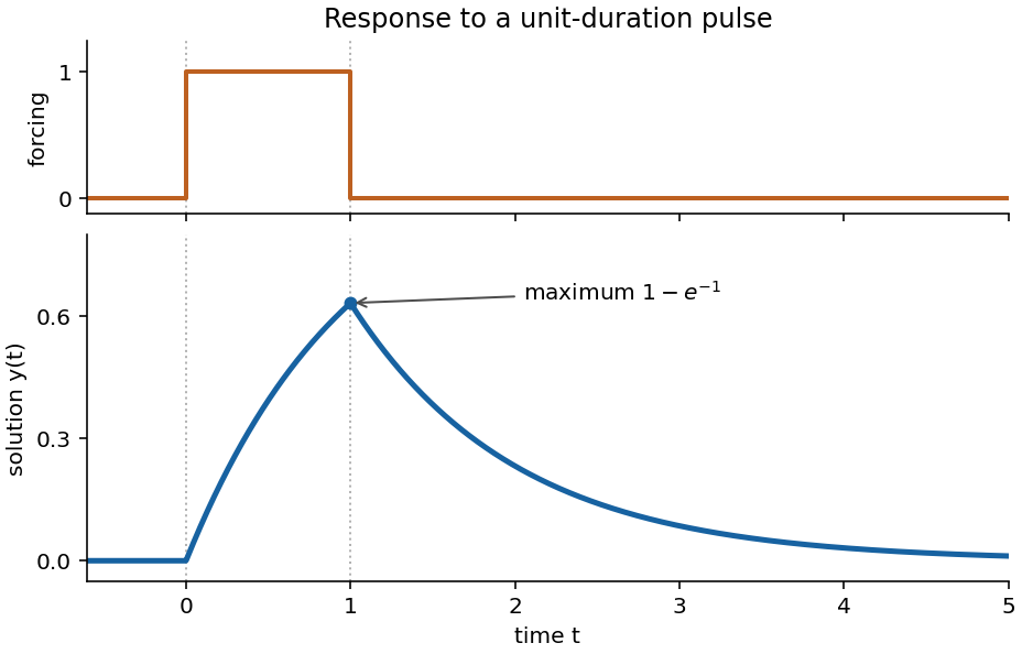
The forcing is a unit pulse on . For , the homogeneous equation and continuity with give . On , integration with gives . At the end of the pulse its value is , and the subsequent homogeneous decay must start at that value. ThusEquivalently it is the difference of two translated step responses, . The solution is continuous, rises concavely to its maximum at , and then decays exponentially to zero. Its derivative has jumps at the pulse edges; those are permitted because the right-hand side has step discontinuities.

For the homogeneous linear recurrence relation, a trial gives the characteristic equation of a linear recurrence . Thus the two homogeneous sequences are and . Seek a particular solution ; substitution gives , so and . HenceThe two independent constants supply arbitrary initial values for this second-order linear recurrence relation.
The homogeneous sequences are again and . A particular solution has left-hand side , so . Consequently . The two initial conditions require and , giving and . ThusThe linear recurrence relation can be rearranged as . Starting with the two integer values, mathematical induction proves that every for is an integer. For , the closed form givesThe first term on the right is divisible by ten; the second is too, because supplies a factor two and supplies a factor five. Therefore divides for every positive integer . The positivity condition matters: at the expression is .
Articles were limited to the first 100 out of 303 total.
Articles by others on the same topic
There are currently no matching articles.