The repeated-root constant-coefficient differential equation has characteristic polynomial . Its two fundamental solutions areThey are linearly independent: their Wronskian is , which never vanishes. For the forced equation, exploit the repeated factor by writing . Direct differentiation gives , so the forcing reduces to . The initial data imply and , hence . ThereforeThe extra factor reflects resonance of the forcing with the repeated characteristic root; the exponential substitution obtains it without guessing a particular solution.
A constant orbit is a fixed point of . Solving gives , henceFor fixed point stability for an iteration, perturb a fixed point by . Its local evolution is , where . At zero, , so perturbations contract: zero is locally asymptotically stable. For example, if , then ; this gives an invariant neighborhood and geometric convergence to zero.
At one, , so perturbations expand: one is unstable. More explicitly, putting gives , whose magnitude increases while a nonzero perturbation remains sufficiently small. The derivative test concerns local stability; it does not assert attraction from every real initial value.
For events with , the conditional probability is . Applying the definition in both orders gives Bayes theorem:Conditionally on , independent fair tosses give a binomial distribution for the head count, so . The joint probability mass function is consequentlyUse the law of total probability and the differentiated geometric series, , to obtain . The posterior coin count after exactly one head is thereforeThese probabilities sum to one by the same series identity. The conditioning weights possible coin counts by their likelihood of producing exactly one head.
For a nonnegative integer-valued random variable, the probability generating function iswith always allowed. Its derivative at from below gives the expectation when finite.
The waiting time has the positive-integer geometric distribution . For the capped geometric waiting time, exactly when , while occurs whenever . Thus the terminal mass is , givingThe finite sum is a polynomial; any apparent singularity of the rational expression is removable. This includes , where .
Differentiating the rational form at yieldsAs a second interpretation, the expectation is the sum of the tail probabilities for . Their finite geometric sum gives the same answer.
Use a power-series solution of a differential equation, . Comparing coefficients givesIn particular , while and are free. The two prescribed derivative pairs select and . The next coefficients are , , , . HenceThese are the first three nonzero terms when the respective parameter is nonzero; if or , the corresponding solution vanishes identically.
For closed forms, set . Cancellation of the first-derivative terms reduces the equation, for , to . The analytic solutions extend across zero, and their hyperbolic cosine and hyperbolic sine expansions identifyThis is the hyperbolic reduction of a regular-singular differential equation: although the original leading coefficient vanishes at zero, both selected power-series solutions of a differential equation are entire.
Completing squares reveals the geometry of the sheared quartic double-well gradient flow:The critical points satisfy and , so they are , and . The Hessian matrix isAt the origin its determinant is , so is a saddle point, with . At either other critical point, the determinant is and the upper-left entry is , so it is a positive-definite matrix. They are strict local minima; the completed squares show that both are global minima, with .
A contour at level obeysThere are no contours for , two isolated minimum points for , and two separate closed ovals for . At the two lobes meet at the saddle point; near the origin their tangents are . For one closed contour surrounds both minima.
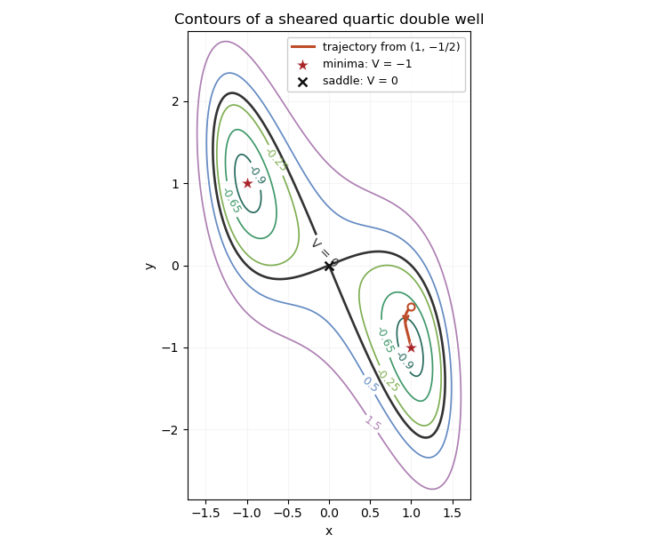
Sheared quartic potential contours and the trajectory to the positive-x minimum
. Along the gradient flow, the gradient-flow dissipation identity isAt the stated initial point, . Its trajectory stays in the invariant sublevel set . This set is compact because is a coercive function. It also excludes every point with , where ; continuity therefore keeps the trajectory in its positive- component.
To justify its limit rather than merely infer it from the sketch, integrate the dissipation identity: is finite. On this compact set the gradient and its time derivative are bounded, so is uniformly continuous. A nonnegative uniformly continuous function with finite integral tends to zero: otherwise separated intervals of a fixed positive height and width would force an infinite integral. Every accumulation point is consequently a critical point. In the positive- component below this energy level the only one is . Compactness then implies convergence, andThis is a compact gradient-flow trapping criterion; the drawn trajectory illustrates, rather than replaces, the convergence proof.
Write the linear system of differential equations asA homogeneous power solves this Cauchy-Euler differential system precisely when . The eigenvalues are and , with eigenvectors and . The homogeneous solution is therefore .
For a particular solution, put . Then , which gives . At , the two initial conditions become and , so . ThusThe two powers correspond to the two eigenvalues; the lower-degree particular term accounts for the constant forcing. Substitution gives both original right sides and the zero initial data.
For the damped harmonic oscillator, the characteristic roots are . For , the real general solution isIf the frequency parameter is zero, the characteristic root is repeated and the complete limiting basis is , so . No sign restriction on is needed for these formulas, although corresponds to decay.
Before the impulse the zero initial data force . An impulse modeled by the Dirac delta function requires continuity of : a jump in would introduce an unwanted derivative of a delta in . Integrating the equation across then gives the velocity jump .
The causal Green function of a damped oscillator isThe jump conditions give the causal impulse responseHere is the Heaviside step function. For , interpret the quotient continuously as , giving . Both initial values are zero because .
The step response of a damped oscillator is the time integral of its causal Green function of a damped oscillator. Put and define for . Then and its oscillator equation has constant right side . Integrating explicitly givesThis formula applies when . It is a convolution of the causal impulse response with the shifted Heaviside step function, so the response is zero before the forcing starts and has the stated zero initial data.
The integral definition also handles the degenerate parameters without division ambiguities. For ,for , . These are the continuous zero-frequency limits of the step response.
Use the shift derivative of a step response, writing with . Differentiate with respect to the forcing location:The possible delta term vanishes because , while . Therefore, as a distribution and also as the ordinary piecewise response,Moving the start of a unit step differentiates its forcing into a negative impulse. The zero initial conditions and linearity ensure that the corresponding responses obey the same identity, including the zero-frequency cases.
The moment-generating function is at real for which that expectation is finite; . For independent random variables, the joint law factorizes, soThis is the transform form of independence. Its ordinary finite-valued interpretation applies where both factors are finite, with the transform of a zero multiple equal to .
Finiteness of the moment-generating function on an open neighborhood of zero gives its differentiability there. Using the permitted interchange of differentiation and expectation,Hence , and . The second-order Taylor expansion with its Peano remainder givesHere is the raw second moment, not the variance: . This distinction matters before specializing to a centered variable.
Let and . Since they are independent, applying the product rule for moment-generating functions to givesAll factors are finite and strictly positive for every real by the stated hypothesis. Applying the same identity to and dividing yields , orThe centered unit-variance Taylor expansion from part (ii) gives and the same expansion for . Consequently .
For the first step of dyadic rigidity of a moment-generating function, take logarithms, which are allowed because . For each fixed and every integer ,Since , the right side tends to zero: it is . Thus for every , and the moment-generating function is even.
The original identity now becomes . Iterating this time with the correct fourth-power scaling givesNear zero, , so the right side tends to . ThereforeThis is the moment-generating function of a standard normal variable. By the uniqueness theorem for moment-generating functions, each of and has the standard normal distribution. The proof establishes the Gaussian characterization by independent sum and difference directly from the two functional identities and the first two moments.
The cumulative distribution function is . For the differentiable distribution in the question, its probability density function is , so probabilities over intervals are obtained by integrating . The survival probability is . Differentiating immediately givesThe strict inequality is consistent with the definition using . This relation connects the probability density function with the decline of the survival probability.
The independent uniform distributions give a constant joint probability density on the unit square. For , integrate over :For the random quadratic with uniform coefficients, real roots require its discriminant to be nonnegative, equivalently . The boundary has probability zero, and the area under this parabola isOn that event the roots are , both nonpositive. Bounding both absolute values by one therefore amounts to bounding the more negative root:Since , squaring the inequality is legitimate and gives . The admissible unit-square region is . Its probability isDividing by the real-root probability gives the requested conditional probability:
For a Galton-Watson process, condition on the number of children of the initial individual. The descendants of these children over the next generations are independent copies of . The probability generating function of their total, conditional on , is . Averaging over the family-size law givesThis is the branching-process generating-function iteration. Conditioning instead on the last generation gives ; both orders agree because is the th iterate of the same function . The argument holds on the usual PGF domain , with larger domains available when the corresponding expectations converge.
The geometric family law on the nonnegative integers has probability generating functionIts expected value is , so this is a geometric-offspring critical branching process. Starting from , verify the rational iterate by induction. If , thenwhich has the same form with replaced by . Thus, for ,The stated disk is the actual power-series convergence domain, not merely a place where the rational continuation can be evaluated. Its simple pole is at .
The extinction probability at generation is the constant coefficient:For later use, expanding the remaining geometric series givesIn particular . At the initial population is one deterministically; its PGF is , and the displayed radius involving is used only for .
For , substitute in the probability generating function. The moment-generating function of isThe domain follows from convergence of the generating series; at or above that positive threshold the expectation diverges, even though a rational continuation can be written.
Conditioning on survival, the probability mass function from part (ii) becomes a positive-integer geometric distribution:Its conditional moment-generating function is , tending to for fixed . We can prove the required limit directly, without invoking a continuity theorem. Set . For every , the strict upper tail is exactlySince and ,At both tails equal one. This is the exponential limit of surviving geometric branching. Conditioning is essential: the unconditional variable has probability of being zero, whereas the rare surviving population has size of order .
For independent random variables, and . Factor their probabilities to obtain the distribution functions of independent minima and maxima:These formulas also allow atoms; no probability density function assumption is needed.
For independent unit-rate exponential distributions, for , so . To establish the independent minimum and gap of two exponential variables, set . On either ordering branch, the change of variables is or with unit absolute Jacobian determinant. Both contribute ; ties have probability zero. Thus the joint probability density isIt factors into normalized exponential probability density functions, proving , and their independence.
The maximum is . A half-scaled unit-rate exponential has rate two, so the independent pair has the same joint law as . ConsequentlyUsing the expected values, variances and independence of the summands,The spacing factorization explains why an order statistic can be represented as a sum of independent waiting times.
Articles by others on the same topic
There are currently no matching articles.