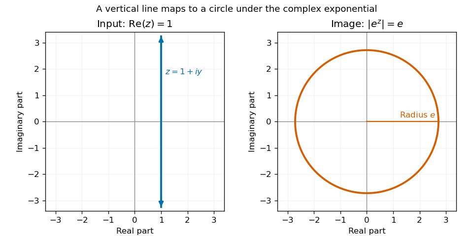
Write with . In the complex plane, this is the vertical line through . The complex exponential gives , so its complex modulus is always . Conversely, every point of that modulus has an complex argument and is obtained in this way. The image is the entire circle centered at zero with radius , traversed repeatedly as varies; it is not a disk.
For , the complex exponential has complex modulus . Equality to the positive real number therefore forces and . The latter holds precisely when is an integer multiple of . Hence all solutions areSubstitution verifies every listed value; the modulus and angle arguments exclude any others.
Let denote the value of the complex logarithm used in the equation. Factoring gives or . Since , the complete answer isThe principal complex logarithm takes exactly these values at and , so both are solutions with that convention. If the complex logarithm is interpreted as multivalued, the same answer holds in the sense that a logarithm value satisfies the equation. The equation is not an assertion that every logarithm value of these numbers has the stated square.
Put . Comparing imaginary parts gives , so . Comparing real parts then gives . The left side is positive, so squaring is legitimate only with , but even then it would give . This contradiction proves there is no solution. Equivalently, with nonzero imaginary part the complex modulus is strictly greater than the real part.
All the transformations below fix the origin. A planar rotation preserves lengths and angles and turns every vector through one common oriented angle. Its rotation matrix isAn orthogonal reflection in a line fixes that line and reverses its perpendicular direction; reflection in the horizontal axis has reflection matrix . A uniform dilation multiplies every vector by the same positive scale , represented by ; for example doubles lengths. A shear mapping fixes one line pointwise and shifts vectors parallel to that line by an amount proportional to their transverse coordinate. A horizontal shear mapping has matrixwith a nontrivial example.
The first given matrix is the clockwise planar rotation through , namely . Direct multiplication givesThus is a horizontal shear mapping of strength . Because ,So is the composition of that shear mapping followed by an anticlockwise planar rotation through ; order matters. It is not individually one of the four elementary types under these definitions. In particular, its determinant is , but it is not an orthogonal matrix, excluding both a planar rotation and an orthogonal reflection. It is not a scalar matrix, excluding a uniform dilation; its eigenvalues and exclude a pure shear mapping, whose eigenvalues are both . As a symmetric positive-definite matrix, can also be described as stretching two perpendicular principal directions by these reciprocal factors, preserving area.
A continuous function at satisfies the following quantified condition:The choice of may depend on and .
For the bounded example, takeThis is a continuous function on its domain and . Along its values tend to , while along its values tend to . Hence the supremum is and the infimum is , and neither is attained. “Upper and lower bound” here means the least upper and greatest lower bounds.
For the nonnegative function on the whole real line, if the conclusion is immediate. Otherwise choose with . The limits at both infinities give such that whenever . By the extreme value theorem, a continuous function on the compact interval has a maximum there. Since , it also exceeds every value outside this interval. Thus is bounded above and attains its global maximum. Nonnegativity ensures that either the function is zero or such a positive comparison value exists; without it, a function such as would have an unattained supremum of zero.
The extreme value theorem ensures that is finite. Since and , multiplication preserves the inequality. Monotonicity of the Riemann integral gives the required boundTo prove the weighted mean value theorem for integrals, put and . If , then , so any works. This includes .
If , the extreme value theorem gives and . Integrating gives . A continuous function on an interval takes every value between its minimum and maximum by the intermediate value theorem. Choose with . Consequently
For a point on the plane, the Cauchy-Schwarz inequality gives , because is a unit vector. Equality is achieved at . Thus the distance from the origin is .
Let and let be the perpendicular projection of the sphere's center onto the plane. Every point of the plane has form with . The Pythagorean theorem givesIf , the sphere equation therefore forces . There is exactly one contact point, ; it lies on both surfaces.
Write . The nonzero scalar triple product proves that are linearly independent, so they form a positively oriented basis of and define a nondegenerate tetrahedron.
For the three faces through the origin, choose the inward unit vectorsTheir signs are correct because each has positive inner product with the opposite vertex vector. Write the center as . It lies on the interior side of every face. Tangency of the interior sphere therefore means signed distance , not , from each of those three planes. Taking inner products givesSolving proves the center formulaThis is the sphere center from three tetrahedron face distances; the interior hypothesis selects these signs rather than an exterior center.
Finally set . The scalar triple product identities give . In particular , and the plane through the three vertices isThe second formula follows by normalizing to a unit vector and applying the first distance result.
The system of linear equations is consistent precisely when belongs to the column space of . If is one solution, all solutions form the affine subspacebecause subtracting two solutions produces a vector in the kernel, and adding any kernel vector preserves the equation. Therefore the necessary and sufficient cases are:
- No solution: , equivalently is outside the column space.
- Exactly one solution: , equivalently ; then for every .
- Infinitely many solutions: . The rank-nullity theorem gives a nonzero kernel vector , and gives distinct solutions for all real .
For the matrix equation, each column of solves the same system of linear equations with the corresponding column of . Thus a unique exists if and only if is invertible, and then . Necessity does not depend on : if is singular and one exists, put any nonzero kernel vector in one column of a matrix and zeros in its other columns. Then and every is another solution.
For the specified data, . If denotes row of and row of , row elimination yields , , and . HenceMultiplying gives the prescribed , which both checks the arithmetic and confirms the unique answer.
Expansion along the first column gives the characteristic polynomialThus the eigenvalue has algebraic multiplicity two. Solving gives and then , leaving arbitrary. Its eigenspace is and has geometric multiplicity one. A diagonalisable matrix needs an eigenvector basis, so is not diagonalisable.
If with invertible, then . Multiplicativity of the determinant givesThe roots of the characteristic polynomial, counted with their multiplicities, are the eigenvalues with their algebraic multiplicities. Thus similar matrices have the same eigenvalues with the same algebraic multiplicities.
The converse is false. The matricesboth have characteristic polynomial , but every matrix similar to is , whereas . Alternatively, their geometric multiplicities for differ.
The Cayley-Hamilton theorem says that every square complex matrix satisfies its own characteristic polynomial: if , thenFor a diagonalisable matrix, write with . The characteristic polynomial is , including repeated roots. Evaluating it at gives zero in each diagonal position, and polynomial evaluation respects matrix similarity: . This proves the requested case.
For the final assertion, let be any complex eigenvalue of , with nonzero eigenvector . From we obtain , so . The characteristic polynomial of this nilpotent linear map is therefore . Applying the full Cayley-Hamilton theorem yields . This argument does not assume is diagonalisable.
The symmetry between the last two coordinates gives the eigenvector with eigenvalue . On vectors , the remaining eigenvalue equation iswhose characteristic polynomial is . Corresponding eigenvectors are and . Thus all eigenvalues and eigenspaces areNonzero scalar multiples give all eigenvectors in each eigenspace. The three displayed vectors are mutually orthogonal and have squared norms , respectively.
The quadratic expression is . Normalize the preceding eigenvectors to obtain an orthonormal basisWith the orthogonal matrix and coordinates , the surface equation becomes . All coefficients are positive, so it is an ellipsoid, with principal semiaxes along the respective eigenvectors. This is principal-axis reduction of a quadric.
A map to the unit sphere is . One explicit matrix isIndeed , so . Since is invertible, every point on the unit sphere has a preimage on the ellipsoid; the map is onto, not merely into. The requested is not unique, since an additional orthogonal matrix on the left preserves the unit sphere.
For a real orthogonal matrix, . ConsequentlyThus it preserves every real inner product, and in particular lengths and angles.
An eigenvalue can be complex even though is real, so use the complex Hermitian inner product. For a nonzero complex eigenvector , the real orthogonal matrix also satisfies . Henceand . Taking complex conjugates in gives because is real. The conjugate vector is nonzero, so .
For the unheaded geometrical conclusion, the third eigenvalue of must be real: nonreal eigenvalues of a real matrix occur in conjugate pairs. Its modulus is one, so it is or . Exact algebraic multiplicity two for excludes a third , leaving . By the supplied diagonalisability fact, the -eigenspace is a two-dimensional plane and the -eigenspace is a line. They are orthogonal: preservation of the inner product between a fixed vector and a negated vector gives . Therefore is the orthogonal reflection in its fixed plane. It fixes the two tangential directions and reverses the normal direction; with unit normal , .
A sequence converges to precisely whenFor a finite collection of convergent sequences, choose for the same tolerance in row , and let . If , every available lies within of , and so does any selected . Every such finite rowwise selection converges to . The finiteness is what permits a single maximum of the cutoffs.
For the infinite collection, defineFor every fixed , this sequence is eventually exactly , and hence converges to . But its diagonal selection is , which has two distinct subsequential limits and does not converge. A moving row index can always choose the exceptional entry before that row reaches its eventual behavior.
The arithmetic-geometric mean inequality givesBy induction these inequalities hold at every step, so is increasing and bounded above by , while is decreasing and bounded below by . The bounded monotone sequence theorem gives limits with . Taking limits in the arithmetic mean recurrence gives , whence . Thus both sequences converge to the same positive limit, the arithmetic-geometric mean iteration's limit. No elementary closed formula for that limit is needed.
Let and suppose . Telescoping givesTo justify the Cesaro mean limit directly, choose so that for . The finite initial sum contributes at most , which tends to zero. The remaining terms contribute at most , and replacing by contributes . Consequently .
Take . Then , but alternates between and . Thus convergence of the scaled sequence does not imply convergence of its successive differences.
No. Take . For each fixed positive integer ,by continuity of the logarithm at . Yet , so is not a convergent sequence of real numbers. Vanishing differences at every fixed lag do not control the accumulation of many small increments.
Yes. The arbitrary variable-lag condition forces the Cauchy sequence property. Suppose otherwise. Then some has the property that, for every , there exist with . In particular, for each , choose such . By the triangle inequality, at least one satisfies or . That index must be strictly greater than , since the difference at itself is zero.
It follows that the following positive integer is defined for every :For this particular function, for every , contradicting the assumed limit zero. Therefore is a Cauchy sequence, and the completeness of the real numbers proves it converges to a finite real limit. This is convergence from arbitrary variable-lag increments; the quantifier over every function is much stronger than the fixed-lag condition in the previous part.
Fix and put , . Then . The bounded monotone sequence theorem gives a limit . If , it lies in the domain, where continuity allows passage to the limit in the recurrence: . That is a fixed point, contrary to . Hence . Continuity is used at a possible positive limiting point, not at the excluded endpoint zero.
No: pointwise convergence need not be uniform convergence. The continuous function maps into itself and is strictly below the identity. Its iteration of a map givesFor every finite , these values tend to as , so . With , choosing gives . Thus no single iterate works for every starting point, although each fixed starting point tends to zero.
Use the discontinuous exampleIn both pieces . For , the image stays strictly above , and induction givesThis positive limiting point is not a fixed point, since . The discontinuity is precisely why the limit cannot be passed through . Therefore the pointwise zero-limit conclusion can fail without continuity.
No: there need not be even one orbit tending to zero. Partition the domain into the disjoint intervalsand, for the unique with , defineThe left endpoint is strictly below , so . Moreover and , so remains in the same interval. For every iterate,Every starting point belongs to some finite-index interval, so this proves the claim for all . The open left endpoints matter: an orbit approaches a boundary but never crosses it. This is discontinuous trapping of decreasing iterates, not a violation of the bounded monotone sequence theorem; each orbit does converge, just to a positive value where continuity fails.
For a series with , suppose exists, allowing . The ratio test says the series converges if and diverges if . In the first case an eventual ratio bound by some compares the tail to a geometric series. In the second case an eventual ratio above some prevents the terms tending to zero.
If , the test is inconclusive: both and have limiting ratio one, while the first diverges and the second converges. If the ratio has no limit, this particular limit formulation gives no conclusion.
The radius of convergence of a power series is the extended real number characterized by absolute convergence for and divergence for . Equivalently,For , only the central point is guaranteed; for , every real point is inside. At finite endpoints , convergence must be investigated separately and is not determined by .
Let be the two radii of convergence. First take , with . Absolute convergence at bounds the terms: for all . ThusAt the right-hand series is finite. Otherwise it converges by the ratio test, because its limiting ratio is . So the differentiated power series converges absolutely at every interior point of , proving . This proof also covers by choosing a finite above any given ; if , that inequality is automatic.
Conversely, if , absolute convergence givesThe constant term does not affect convergence, and both series converge at zero. Hence , including the zero and infinite cases. Therefore . This proof uses coefficient estimates, rather than assuming the termwise differentiation of a power series result whose radius assertion is being established.
The termwise differentiation of a power series theorem states that inside its radius of convergence, the sum is differentiable and its derivative is the sum of the differentiated series. Accordingly . There is no blanket differentiability assertion at the convergence endpoints.
For any fixed real , the ratios between consecutive nonzero terms in the absolute-value series areandThe ratio test proves absolute convergence of both power series at every such ; convergence at zero is immediate. Both radii of convergence are therefore . Applying the test to the nonzero terms avoids the undefined coefficient ratios caused by alternate zero coefficients when these are viewed as full power series in .
Since the common radius of convergence is infinite, the termwise differentiation of a power series theorem applies on the entire real line. For the even series, differentiation and the index change giveThe odd series similarly gives . Thus everywhere. By the product rule,The mean value theorem implies that a differentiable function with zero derivative is constant on the real line. At zero, the series give and . Consequently . This derives the identity from the power series without assuming a trigonometric identity in advance.
The repeated-root constant-coefficient differential equation has characteristic polynomial . Its two fundamental solutions areThey are linearly independent: their Wronskian is , which never vanishes. For the forced equation, exploit the repeated factor by writing . Direct differentiation gives , so the forcing reduces to . The initial data imply and , hence . ThereforeThe extra factor reflects resonance of the forcing with the repeated characteristic root; the exponential substitution obtains it without guessing a particular solution.
A constant orbit is a fixed point of . Solving gives , henceFor fixed point stability for an iteration, perturb a fixed point by . Its local evolution is , where . At zero, , so perturbations contract: zero is locally asymptotically stable. For example, if , then ; this gives an invariant neighborhood and geometric convergence to zero.
At one, , so perturbations expand: one is unstable. More explicitly, putting gives , whose magnitude increases while a nonzero perturbation remains sufficiently small. The derivative test concerns local stability; it does not assert attraction from every real initial value.
For events with , the conditional probability is . Applying the definition in both orders gives Bayes theorem:Conditionally on , independent fair tosses give a binomial distribution for the head count, so . The joint probability mass function is consequentlyUse the law of total probability and the differentiated geometric series, , to obtain . The posterior coin count after exactly one head is thereforeThese probabilities sum to one by the same series identity. The conditioning weights possible coin counts by their likelihood of producing exactly one head.
For a nonnegative integer-valued random variable, the probability generating function iswith always allowed. Its derivative at from below gives the expectation when finite.
The waiting time has the positive-integer geometric distribution . For the capped geometric waiting time, exactly when , while occurs whenever . Thus the terminal mass is , givingThe finite sum is a polynomial; any apparent singularity of the rational expression is removable. This includes , where .
Differentiating the rational form at yieldsAs a second interpretation, the expectation is the sum of the tail probabilities for . Their finite geometric sum gives the same answer.
Use a power-series solution of a differential equation, . Comparing coefficients givesIn particular , while and are free. The two prescribed derivative pairs select and . The next coefficients are , , , . HenceThese are the first three nonzero terms when the respective parameter is nonzero; if or , the corresponding solution vanishes identically.
For closed forms, set . Cancellation of the first-derivative terms reduces the equation, for , to . The analytic solutions extend across zero, and their hyperbolic cosine and hyperbolic sine expansions identifyThis is the hyperbolic reduction of a regular-singular differential equation: although the original leading coefficient vanishes at zero, both selected power-series solutions of a differential equation are entire.
Completing squares reveals the geometry of the sheared quartic double-well gradient flow:The critical points satisfy and , so they are , and . The Hessian matrix isAt the origin its determinant is , so is a saddle point, with . At either other critical point, the determinant is and the upper-left entry is , so it is a positive-definite matrix. They are strict local minima; the completed squares show that both are global minima, with .
A contour at level obeysThere are no contours for , two isolated minimum points for , and two separate closed ovals for . At the two lobes meet at the saddle point; near the origin their tangents are . For one closed contour surrounds both minima.
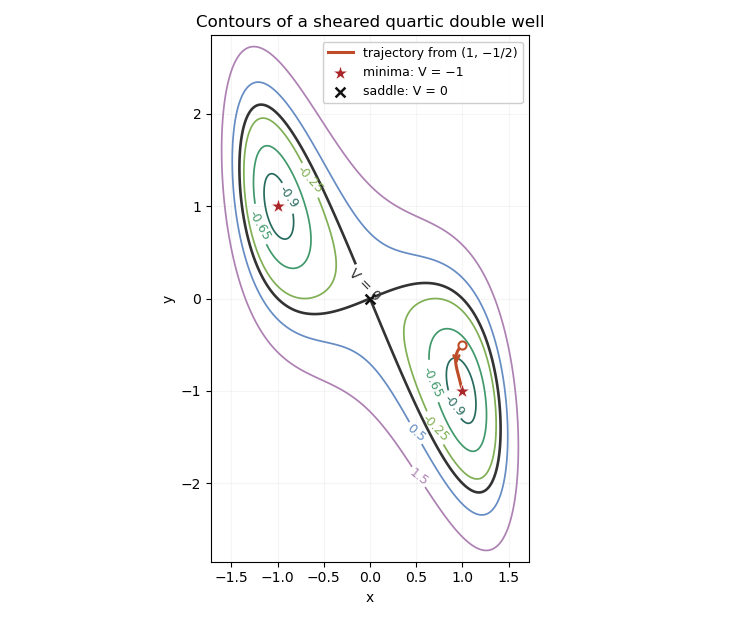
Sheared quartic potential contours and the trajectory to the positive-x minimum
. Along the gradient flow, the gradient-flow dissipation identity isAt the stated initial point, . Its trajectory stays in the invariant sublevel set . This set is compact because is a coercive function. It also excludes every point with , where ; continuity therefore keeps the trajectory in its positive- component.
To justify its limit rather than merely infer it from the sketch, integrate the dissipation identity: is finite. On this compact set the gradient and its time derivative are bounded, so is uniformly continuous. A nonnegative uniformly continuous function with finite integral tends to zero: otherwise separated intervals of a fixed positive height and width would force an infinite integral. Every accumulation point is consequently a critical point. In the positive- component below this energy level the only one is . Compactness then implies convergence, andThis is a compact gradient-flow trapping criterion; the drawn trajectory illustrates, rather than replaces, the convergence proof.
Write the linear system of differential equations asA homogeneous power solves this Cauchy-Euler differential system precisely when . The eigenvalues are and , with eigenvectors and . The homogeneous solution is therefore .
For a particular solution, put . Then , which gives . At , the two initial conditions become and , so . ThusThe two powers correspond to the two eigenvalues; the lower-degree particular term accounts for the constant forcing. Substitution gives both original right sides and the zero initial data.
For the damped harmonic oscillator, the characteristic roots are . For , the real general solution isIf the frequency parameter is zero, the characteristic root is repeated and the complete limiting basis is , so . No sign restriction on is needed for these formulas, although corresponds to decay.
Before the impulse the zero initial data force . An impulse modeled by the Dirac delta function requires continuity of : a jump in would introduce an unwanted derivative of a delta in . Integrating the equation across then gives the velocity jump .
The causal Green function of a damped oscillator isThe jump conditions give the causal impulse responseHere is the Heaviside step function. For , interpret the quotient continuously as , giving . Both initial values are zero because .
The step response of a damped oscillator is the time integral of its causal Green function of a damped oscillator. Put and define for . Then and its oscillator equation has constant right side . Integrating explicitly givesThis formula applies when . It is a convolution of the causal impulse response with the shifted Heaviside step function, so the response is zero before the forcing starts and has the stated zero initial data.
The integral definition also handles the degenerate parameters without division ambiguities. For ,for , . These are the continuous zero-frequency limits of the step response.
Articles were limited to the first 100 out of 221 total.
Articles by others on the same topic
There are currently no matching articles.