Set and for spatial indices. The complex conjugation of the scalar supplies a minus sign, while conjugating each of the three spatial gamma matrices supplies three more. In the original order,Consequently the chirality matrix obeysNo rearrangement of the gamma matrices is needed, so no additional anticommutator sign occurs. The star is entrywise complex conjugation, not matrix transpose or Hermitian conjugation.
Assume a complete relativistically normalized basis of scalar momentum eigenstates transforms asThis states both reversal of spatial momentum and preservation of the normalization of basis quantum states. Antilinearity alone would not suffice: multiplying a conjugation operator by two gives an antilinear operator that multiplies squared norms by four.
Expand and similarly for , with . This Lorentz-invariant phase-space measure is unchanged under . The antilinearity of the quantum time-reversal operator gives conjugated expansion coefficients. Orthogonality of the momentum eigenstates and cancellation of their unit-modulus phases yieldSince momentum reversal is a bijection of the complete basis, is also onto. ThusThis proves antiunitarity, with the normalization hypothesis explicitly included. For scalar multiparticle quantum states the same argument uses the complete occupation-state basis and reverses all momenta; it is not restricted to a single-particle wave packet.
Write for , so . Under the antiunitary operator , the coefficients and exponentials in the mode expansion of a Dirac field are conjugated as well as the creation and annihilation operators being transformed. ThusRelabel and . The stated Dirac spinor identities implyAlso . Substitution reconstructs the original Dirac field at the reflected time:The minus sign comes from reversing the spin label, not from anticommuting field operators. This is the relation between the time-reversal matrix and the charge-conjugation matrix in the supplied spin phases and intrinsic phase convention. Rephasing the charge-conjugation matrix or the intrinsic time-reversal phase can change its displayed form. It proves time reversal of a Dirac field without identifying an antiunitary operator with its finite-dimensional spinor matrix.
Use without summing in individual component transformations. The Dirac current transforms asSince the coupling is real, invariance of its contraction fixes the time reversal of an electromagnetic gauge field:These equations use a compatible gauge; an additional pure gauge transformation would not change the gauge field strength.
Coordinate differentiation at introduces , because the time coordinate is reversed and the spatial coordinates are unchanged. HenceThus the electric field is even and the magnetic field is odd. The chirality matrix is even by part (a). The two tensor signs cancel in the dipole contraction, but antiunitarity conjugates its explicit . Therefore the time-reversal parity of a fermion electric dipole operator isIt is a time-reversal symmetry violating interaction, and, under the usual local relativistic quantum field theory hypotheses of the CPT theorem, it violates CP symmetry. A nonzero coefficient is absent from the renormalizable tree-level Standard Model Lagrangian: the broken-phase fermion electric dipole moment operator has mass dimension five, and its electroweak-invariant completion requires a Higgs field and has dimension six. However, it can arise as a radiatively induced effective interaction in the Standard Model, whose CKM matrix contains a CP-violating phase. It is not forbidden to all orders. An explicit primary calculation of quark dipoles is Czarnecki and Krause's Standard Model calculation.
Starting from a matter-antimatter symmetric ensemble, exact charge conjugation would pair every baryon-producing process with an equally probable antibaryon-producing process. Their contributions to the net baryon number cancel. Thus C violation is necessary. Violating charge conjugation alone is insufficient: if CP symmetry is exact, the parity-reflected conjugate channels still have equal probabilities and cancel in a CP symmetry invariant ensemble. One needs CP violation as well.
The remaining Sakharov conditions are baryon number violation and departure from thermal equilibrium. Conserving baryon number cannot turn an initially zero value into a nonzero one. In thermal equilibrium, under the usual CPT theorem hypotheses and with no imposed chemical potentials for charges odd under CPT symmetry, states and their conjugates have equal thermal weights, so the equilibrium expectation of net baryon number vanishes and thermal stationarity prevents its sustained production. A nonequilibrium history allows different forward and reverse populations to generate an asymmetry. These are the standard necessary conditions for dynamical baryogenesis from symmetric initial conditions, not a guarantee of a sufficiently large asymmetry.
Take , , metric , and a Higgs potential with , . The gauge-scalar electroweak interaction isHere . With the printed plus-sign convention for , define ; thus . The minus sign in the nonlinear gauge field strength follows from this convention.
The minima have , with . A gauge transformation rotates the vacuum to . In unitary gauge, the three angular Goldstone bosons are removed, leaving and one real Higgs boson. The generator annihilates the vacuum, because its lower component has and hypercharge . This identifies the unbroken electromagnetic gauge group.
The quadratic terms from the Higgs field kinetic term areDefine the Weinberg angle and physical fields byThe neutral combinations areThe neutral gauge-boson mass matrix is . It has eigenvalues zero and , with the zero eigenvector giving . Expanding the Higgs potential about its minimum gives . Therefore the tree-level electroweak gauge-boson masses and scalar mass areAlso and . The three removed Goldstone bosons supply the longitudinal polarization vector degrees of freedom of the massive electroweak gauge bosons.
Replacing by in the neutral mass term gives all the Higgs boson couplings to Z bosons in unitary gauge:There are exactly the cubic and quartic elementary tree-level Feynman diagrams. Differentiating with respect to the identical fields gives Feynman rules and , respectively. There is no elementary vertex for the real neutral radial field.
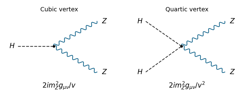
Higgs interaction vertices
. The two elementary Higgs boson couplings to Z bosons, with dashed scalar legs and wavy vector legs. Details.
The authoritative PDF has , not the dimensionally incorrect in the TeX conversion. The two identical Z bosons give the vertex factor two, so the scattering amplitude for the decay isup to an irrelevant overall phase. Apply the massive vector polarization sum, identifying the hint's with :Since , putting givesNo initial-spin average is needed for a Higgs boson. In its rest frame the two-body momentum is . Integrating the energy and momentum delta functions in the Lorentz-invariant phase-space measure gives , hence .
The printed generic width formula treats the daughters as labelled. Here the identical final-state symmetry factor is , without which the same physical configuration is counted twice. Thus the Higgs decay to two Z bosons hasEquivalently, gives the prefactor . The threshold limit is zero and the large-mass limit is . The additional factor for identical daughters is a required specialization of the PDF's generic phase-space formula, not an extra factor in the vertex.
The three allowed tree-level Feynman diagrams are shown below, using physical-particle Feynman propagators in unitary gauge. Solid arrows follow fermion number and the wavy lines denote the charged vector Feynman propagator.
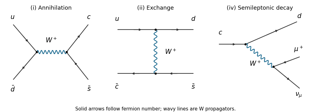
Charged-current interaction diagrams
. The allowed s-channel, t-channel and semileptonic weak charged current graphs. Details.
Allowed through an s-channel W boson. The initial up quark and down antiquark annihilate into a virtual , which produces the final charm quark and strange antiquark. The two weak charged current vertices contain the nonzero CKM matrix elements and , with complex conjugations determined by fermion-flow conventions.
The left panel shows the unique physical-particle tree-level Feynman diagram. A neutral exchanged gauge boson cannot connect these charged annihilation currents, and flavour-diagonal neutral vertices cannot turn an up quark into a charm quark. There is no additional elementary charged scalar in the minimal Standard Model.
Allowed through a t-channel W boson. Along one fermion line the up quark becomes a down quark by emitting a virtual ; along the other the charm antiquark absorbs it and becomes a strange antiquark. The middle panel shows this weak charged current exchange. Both electric charge and baryon number are conserved at each vertex, and the relevant CKM matrix entries are nonzero.
This is the unique physical-particle tree-level Feynman diagram. A neutral exchange would require a flavor-changing neutral current on each line, absent at tree level in the Standard Model. An annihilation into a neutral boson would likewise require an off-diagonal up-type neutral current. The different generations do not forbid the charged-current graph.
Forbidden by electric-charge conservation. The initial bottom quark has electric charge , while the displayed final electric charges sum to . Therefore no Standard Model Feynman diagram, at tree level or any loop order, can realize this channel.
This is an intentionally disallowed process, not a transcription correction. The charge-conserving semileptonic bottom decay instead has an electron and an antineutrino of electron flavour, while a Positron accompanies the conjugate antiquark decay. Replacing the displayed particles silently would change the requested classification.
Allowed through a virtual W boson. The charm quark emits a and becomes a down quark through the nonzero CKM matrix element . The virtual W boson produces a positive muon and a muon neutrino through the leptonic weak charged current. The right panel is the unique physical-particle tree-level Feynman diagram.
Its total electric charge is , equal to the initial charge, and its final lepton number is . The decay is Cabibbo suppressed, rather than forbidden. These diagram counts use unitary gauge: in covariant gauges charged unphysical Goldstone bosons can supply gauge-dependent pieces of the same physical amplitudes, not additional physical channels.
Use metric , and relativistically normalized external spinors. The Fermi interaction givesup to an irrelevant phase. The fermion spin sums replace and by the slashed massless momenta. Write . The gamma matrix trace identities yieldThe symmetric-antisymmetric mixed contractions vanish. The symmetric contraction is , while the two epsilon tensors contract to . Including and the initial-spin average therefore givesThe singlet color charge contractions have net factor one after summing final colours and averaging initial color charge states. Thus this is also the colour-averaged partonic result; no extra factor three is required.
In the centre-of-momentum frame, let . The Mandelstam variables satisfy and , giving and . HenceThe massless invariant flux factor is and , so the weak charged-current quark scattering cross-section isFor a purely left-handed weak charged current, , , this reduces to , fixing the sign of the forward term. Purely right-handed weak charged currents at both vertices have the same unpolarized angular law. The factorization convention for could be rescaled by a common numerical factor; the displayed product fixes the normalization.
For fixed the effective Fermi interaction predicts . The angular odd term integrates to zero, while , soThe corresponding fixed-spin scattering amplitudes grow as , eventually conflicting with partial-wave unitarity. This is a failure of extrapolating the effective field theory, whose contact approximation requires , not a failure of the Standard Model.
Restoring the virtual W boson Feynman propagator replaces its constant low-energy denominator by , away from the resonance. The massless external Dirac equations give zero contraction of each current with the exchanged momentum, so the longitudinal numerator does not contribute. Its squared modulus multiplies the effective cross-section. For the resulting tree-level rate decreases as rather than growing as . Near the pole one must include the W boson decay width. These statements assume the same massless conserved external currents; the contact expression alone is not valid there.
Opposite directions replace by . The even term cancels from the numerator and the odd term from the denominator. For , the angular asymmetry of a chiral charged-current interaction isHere denotes the antipodal direction in the stated angular law. If , both rates vanish and the asymmetry is undefined.
The overall Fermi constant, energy-dependent prefactor and common normalization cancel. Thus this observable constrains the relative vector current and axial current couplings of the weak charged current rather than only their total strength. Pure vector currents or pure axial currents give zero asymmetry; gives the maximal coefficient, . The inequality ensures .
It does not uniquely identify the handedness: the formula is insensitive to , , and interchanging . In particular equally strong purely left- and right-handed weak charged currents at both vertices are indistinguishable in this unpolarized measurement. Additional spin-sensitive observables would be needed to remove that degeneracy. The cancellation and constraints are within the massless parton approximation specified for the calculation.
For positive in the perturbative regime, the sign of the renormalization-group beta function fixes the direction of flow. If , then decreases when the renormalization scale increases: the theory exhibits asymptotic freedom. Toward low scales the interaction grows stronger, and its one-loop approximation reaches an infrared strong-coupling scale. This perturbative divergence does not by itself prove confinement.
If , increases toward the ultraviolet and decreases toward the infrared: the one-loop flow is infrared free and has an ultraviolet Landau pole. Indeedwhose right side reaches zero at a finite ultraviolet scale for negative . Beyond strong coupling this formula is not controlled. If , the displayed one-loop term gives no running and higher orders decide the behavior; is a fixed point in all three cases.
Differentiating the strong coupling constant givesIntegrate this constant derivative and express the integration constant through the strong-coupling scale at which the one-loop inverse coupling vanishes. The one-loop running of the strong coupling isThe positive-coupling branch has and is perturbatively reliable only when the logarithm is sufficiently large. The pole at signals failure of the one-loop expansion, not a prediction of a physically infinite observable. Equivalently, is scale-independent to this order; this is dimensional transmutation.
For the Quantum chromodynamics gauge group , the coefficients on the two sides of the bottom threshold are and . Continuity of the one-loop running of the strong coupling at givesThus matching the QCD scale across a quark threshold yieldsThe scale parameter changes because the beta-function coefficient changes, even though the matched coupling is continuous. This is leading-order matching with a fixed flavour number within each region; the stated four-flavour region is the effective region above the charm threshold, not a literal claim that four quarks remain active down to arbitrarily small scales.
Set , , and , treating as fixed. The notation means the coupling evaluated at energy scale , using the squared-scale label. The one-loop running of the strong coupling gives . Write , so andDifferentiating both explicit and implicit scale dependence givesFor nonzero coupling and , the principle of minimal sensitivity applied to this truncated expression with one-loop running therefore selectsThis is the one-loop stationary scale for the hadronic annihilation correction. For five active flavours it is approximately , or . It is meaningful within a fixed-flavour perturbative region; crossing a threshold requires the appropriate matched coupling.
The derivative cancels identically through order . The prescription retains the residual order- term generated by differentiating the truncated observable with the one-loop running. If one instead discards every order- contribution, no unique scale is determined: every scale is stationary to the retained accuracy. Two-loop running and uncomputed higher observable coefficients can shift the optimum. For , or the trivial limit, this leading approximation likewise selects no unique scale.
Articles by others on the same topic
There are currently no matching articles.