Use the inverse beta decay threshold, with the charged-lepton mass generalized to . For a stationary proton and a massless incident antineutrino, the Mandelstam invariant is . At threshold the final particles have no relative momentum in their centre-of-momentum frame, so . ThereforeUsing the supplied, rounded masses givesThe second term is the recoil correction; setting the threshold equal just to the final rest-mass excess would miss it.
Reactor electron antineutrinos have energies of a few million electronvolts. They can produce a Positron through inverse beta decay above the first threshold, but cannot produce a muon. Thus reactor neutrino oscillations are measured primarily as electron-antineutrino disappearance, through the event rate and energy spectrum relative to the unoscillated prediction. An oscillated muon antineutrino cannot be identified by the proposed muon-production channel at reactor energies; disappearance alone does not distinguish all possible final flavours.
The separate proton and neutron shell capacities are . Filled shells and paired particles have zero net spin and magnetic dipole moment. The single-particle nuclear magnetic moment is , with orbital factors , and .
For nitrogen, the eight neutrons form a closed shell. The seventh proton occupies , so , and the Landé g-factor givesHence the nuclear shell model predictsIts single-particle spin and parity is . The negative moment results from the proton spin being predominantly opposed to the total angular momentum in this level.
For oxygen, eight protons and the first eight neutrons are paired. The ninth neutron occupies , with , . Since its orbital factor is zero, . ThereforeThese are ideal single-particle predictions in units of the nuclear magneton, not fits incorporating nuclear configuration mixing.
For negligible final fermion masses, the chiral Z-boson partial width is proportional to . Both channels have one color state. An Electron has , and , givingFor one active neutrino species, , and there is no coupled right-handed neutrino field, so , . The common coupling normalization and phase space cancel in the ratio:The same total decay width appears in the two branching fractions, soThere is no factor of three for a single specified flavour. Summing three active neutrino flavours would give an invisible branching fraction of approximately in this approximation.
What is measured. A monoenergetic Electron beam is directed at a thin target. A movable magnetic spectrometer selects the scattering angle and outgoing momentum, separating elastic scattering from nuclear excitation and other backgrounds. Incident beam current and target thickness supply the normalization of the differential scattering cross-section. The Hofstadter nuclear electron scattering experiment is a classic implementation of this electromagnetic probe.
For a heavy, approximately spin-zero atomic nucleus, neglecting recoil and treating the electron in the Born approximation, the point-charge result is multiplied by the nuclear charge form factor:Here is the magnitude of the spatial momentum transfer in natural units. The cosine factor includes the Electron spin. Dividing the elastic data by the point-charge factor isolates within these approximations. Recoil, magnetic terms for targets with spin, radiative corrections and particularly Coulomb distortion in electron scattering must be included when significant.
From scattering to size and shape. For a spherical nuclear charge distribution,Thus the nuclear charge form factor is a normalized Fourier transform. Its low- expansion,measures the nuclear charge radius . Larger momentum transfers resolve the density profile through diffraction maxima and minima. For a uniform sphere of sharp radius , the uniform-sphere nuclear charge form factor is ; its first zero is at , while .
A practical extraction fits a family of densities to all measured cross sections, rather than treating a few measured values of as a complete density reconstruction. Finite angular coverage, resolution and the missing sign information make this an inverse problem.
Observed pattern. Apart from the lightest nuclei, the central density is approximately constant; the size grows approximately as and there is a diffuse surface. The coefficient describes an equivalent sharp nuclear radius, rather than the root-mean-square radius itself. Heavy nuclear charge distributions are often described by the two-parameter Fermi nuclear charge distribution, , with half-density radius scaling roughly as and diffuseness around . The surface thickness is then about . Shell effects, deformation and the lightest systems give departures from this smooth pattern. These qualitative features are established by the electron scattering density measurements.[ref]
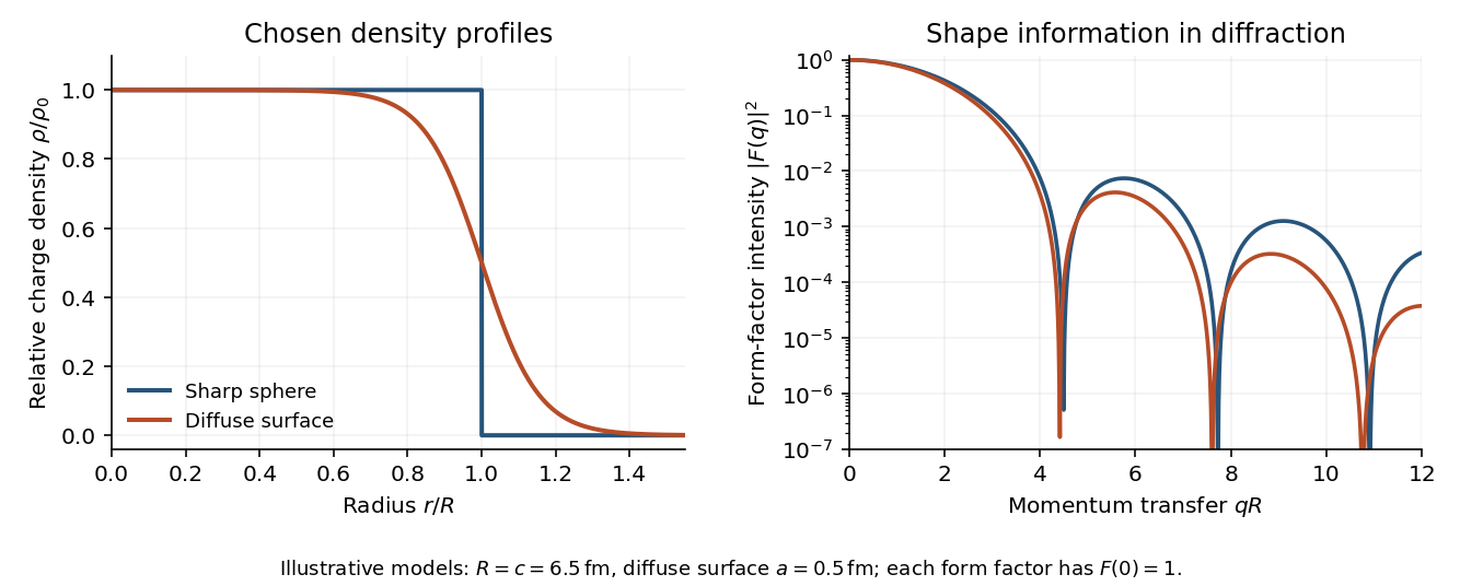
Original sharp-edge and diffuse nuclear charge models, showing how a surface profile changes the nuclear charge form factor
. Details. 
Complementary probes. Transition energies in a muonic atom are especially sensitive to nuclear size because the heavy negative muon orbits close to the charge. Electronic isotope shifts, after separating nuclear-mass and finite-size contributions, measure changes in . Both require atomic-structure calculations. Electromagnetic excitation and transition strengths constrain deformation and charge multipoles. Hadronic scattering can also constrain nuclear dimensions, but carries uncertainties from the strong interaction and probes matter rather than purely electric charge.
Theory. Quantum chromodynamics is a local, non-Abelian gauge theory with gauge group SU(3) acting on color charge. Its matter fields are spin-half quarks of six flavours, each in three colors; its eight massless spin-one gluons are the gauge fields. Unlike the neutral photon, gluons themselves carry gauge charge. Consequently there are three-gluon and four-gluon vertices as well as the quark-gluon vertex. A compact Lagrangian density iswhere is the gauge covariant derivative and the field strength contains the nonlinear term .
The running coupling is weak at high momentum scales. At one loop, for active flavours,The positive coefficient produces asymptotic freedom: short-distance, large- processes admit perturbation theory. The gluon self-interaction is crucial to its sign. At low scales the coupling grows and isolated colored particles are not observed; the physical spectrum consists of color-singlet hadrons, the phenomenon of confinement. A hard-produced quark or gluon radiates and undergoes hadronization, giving a collimated jet. The one-loop formula is not valid at and is not, by itself, a mathematical proof of confinement.
- Deep inelastic scattering resolves approximately pointlike spin-half constituents. Approximate Bjorken scaling supplies the starting parton picture, while the measured logarithmic departures from scaling agree with QCD evolution of parton distribution functions.
- The hadronic R ratio in electron-positron annihilation counts squared quark charges multiplied by three colors, with calculable strong corrections. It tests color multiplicity as well as the quark charge assignments.
- Two-jet events identify a quark-antiquark hard topology. Three-jet events test hard gluon radiation, ; their angular correlations support a spin-one gluon. Four-jet correlations and radiation patterns further probe the non-Abelian color factors and gluon self-interactions.
- Determinations of from processes at widely separated scales follow the same running coupling, rather than independent interaction strengths. Jet rates, event shapes, hadronic weak-boson decays and high-energy hadron collisions provide complementary tests.
- Lattice QCD calculations reproduce many hadronic masses and other low-energy quantities from the same underlying theory, connecting its strongly coupled regime to the observed spectrum.
The convincing evidence is the quantitative consistency across these probes, with a common color group and coupling evolution. A jet by itself is evidence for a hard parton; its rates and correlations supply the more specific tests of Quantum chromodynamics.[ref]
Production and identification. At a hadron collider, initial partons carry fractions of the proton momenta; observable production rates combine parton-level amplitudes with parton distribution functions.
- Top quark pairs are produced through and . Single top production uses the weak charged current, for example through a virtual W boson. The dominant decay is , and similarly for the antiquark. The subsequent W boson decays produce dilepton, lepton-plus-jets and all-hadronic channels. Reconstructing the W and b systems constrains the top mass. The top decays before forming an ordinary long-lived top hadron.
- An on-shell W boson is produced by quark-antiquark annihilation, for example . Other sources include top decay and boson-pair production; at a lepton collider, provides a clean pair channel. The W boson decays to or to a kinematically accessible quark pair. Neglecting masses and strong corrections, the three lepton channels and two up-type quarks with three colors give approximately one-third leptonic and two-thirds hadronic branching. The leptonic modes combine a charged lepton with missing transverse momentum; the transverse-mass distribution constrains .
- Higgs boson production includes gluon fusion through a heavy-quark loop, vector-boson fusion , associated , and production. At a lepton collider, is another example. For a Higgs mass near , important decays include , , , and . The less frequent mode and mode give especially clean reconstructed mass peaks. The asterisk denotes an off-shell daughter boson; two on-shell W or Z bosons are inaccessible at that Higgs mass.
Why the three masses form a test. At tree level, electroweak symmetry breaking gives and . The Higgs mechanism relates masses to the vacuum field, but it does not by itself predict the top Yukawa coupling or the Higgs self-coupling, so the three masses are not fixed independently of measured parameters.
The stronger test comes from radiative corrections. With accurately measured , and , the electroweak precision test with the W, top and Higgs masses usesThe top-bottom loop contributes approximately , while the Higgs contribution has a characteristic logarithmic mass dependence. Hence direct measurements of and turn the precision calculation into a prediction for . Comparing that prediction with the direct W-mass measurement overconstrains the Standard Model; disagreement beyond experimental and theoretical uncertainties could indicate additional particles or interactions in the loops. The test concerns the relation among independently measured quantities, rather than merely the existence of the three particles.
Alpha lifetimes and competing beta decays. The Geiger-Nuttall law follows approximately from quantum tunnelling through the daughter’s Coulomb barrier. Increasing shortens the barrier and greatly increases the decay rate; increasing the daughter charge makes the barrier harder to penetrate. A useful local parametrization isUsing the supplied nuclear masses, no electron-mass subtraction is needed for alpha decay. The calculated Q values areCalibrate the two constants to the two supplied even-even thorium half-lives. Their daughter charges are both 88, soThis gives the order-of-magnitude estimatesHere . The known beta-minus decay rates are approximately and , respectively. Thus the reference alpha branching fractions are only about and . Beta decay overwhelmingly removes the parents before alpha emission, explaining why the alpha branches are not seen in the stated chain.
These estimates are local extrapolations, not precision predictions. In particular, actinium is odd-odd, so extrapolating an even-even Geiger-Nuttall law neglects nuclear-structure and angular-momentum hindrance. Such effects can further suppress its alpha branch.
Allowed daughter spin and parity. The even-even parent in its ground state and the alpha particle both have . The total final angular momentum must be zero, so coupling daughter spin to relative orbital momentum requires . Parity conservation gives . The alpha-decay angular-momentum and parity selection rule is thereforeThese are the natural parity states. Restricting the list to even spin would be too strong; even-spin rotational bands are a further structural specialization.
Ground-state line and recoil. The nuclear alpha-decay recoil correction givesFor the thorium ground-state decay, this predicts , with daughter recoil about . This is close to the highest measured line, : the difference is , or . Conversely that line implies . The quoted nuclear masses have only five decimal places in atomic mass units; rounding three such entries can shift their mass difference by up to about . Thus the requested approximate agreement is supported, but the rounded table does not reproduce the line energy exactly. Dropping daughter recoil would give an error around instead.
Excited levels. Relative to the highest line, the two alpha-energy deficits are and . Multiplying by the common recoil factor givesA deformed even-even nucleus has a ground-state nuclear rotational band with and . Its to excitation ratio is , with the observed ratio about below this ideal value. The likely assignments are therefore and rotational excitations, with modest departures from a rigid constant-inertia rotor. The ratio supports this interpretation; it is not a unique spin measurement by itself.
Sargent comparison. For beta-minus decay using nuclear masses, subtract the emitted electron rest mass:The simple version of Sargent's rule would predictThe measured rate ratio is the inverse half-life ratio,The naive fifth-power estimate is about times larger. It correctly predicts the much faster actinium decay but fails quantitatively. The small radium endpoint is far below the electron rest mass, violating the negligible-mass approximation behind the fifth power; Coulomb distortion of the emitted electron, different nuclear matrix elements and different daughter excitations also matter. The rounded mass difference makes the very small radium especially uncertain. The appropriate comparison of individual branches uses the actual endpoint-dependent statistical factor and comparative half-life, not a universal fifth power of the ground-state release.
Beta selection rules and the four observed branches. The radium parent has , so the ground-state transition is a unique forbidden beta decay of second order: it preserves parity and requires three units of angular momentum. For the increasing daughter excitation energies, the endpoints decrease. The assignments areFor , zero lepton orbital angular momentum and lepton-pair spin one give an allowed beta decay of Gamow-Teller transition type. The branches need odd lepton orbital angular momentum, with lowest value one, and are forbidden beta decays of first order; they are not unique because they do not have the maximal transfer at that order.
The absence of a listed ground-state branch is consistent with its stronger forbiddenness. The two allowed branches carry in total, and the nearly equal-endpoint pair favours the allowed branch by four to one. These trends support the classification. However, first-forbidden branches still carry , and the lower-endpoint first-forbidden branch is stronger than the higher-endpoint one. Thus selection-rule labels alone do not explain all intensities: nuclear overlaps and the endpoint-dependent phase space are indispensable. “Forbidden” means suppressed at leading order, not impossible.
Continuum amplitudes. The leading quantum electrodynamics diagram is electron-positron annihilation into a virtual photon, followed by conversion to a muon pair. Replacing the outgoing muons with a quark-antiquark pair gives the quark-level hadronic diagram. The first two panels below show these processes.
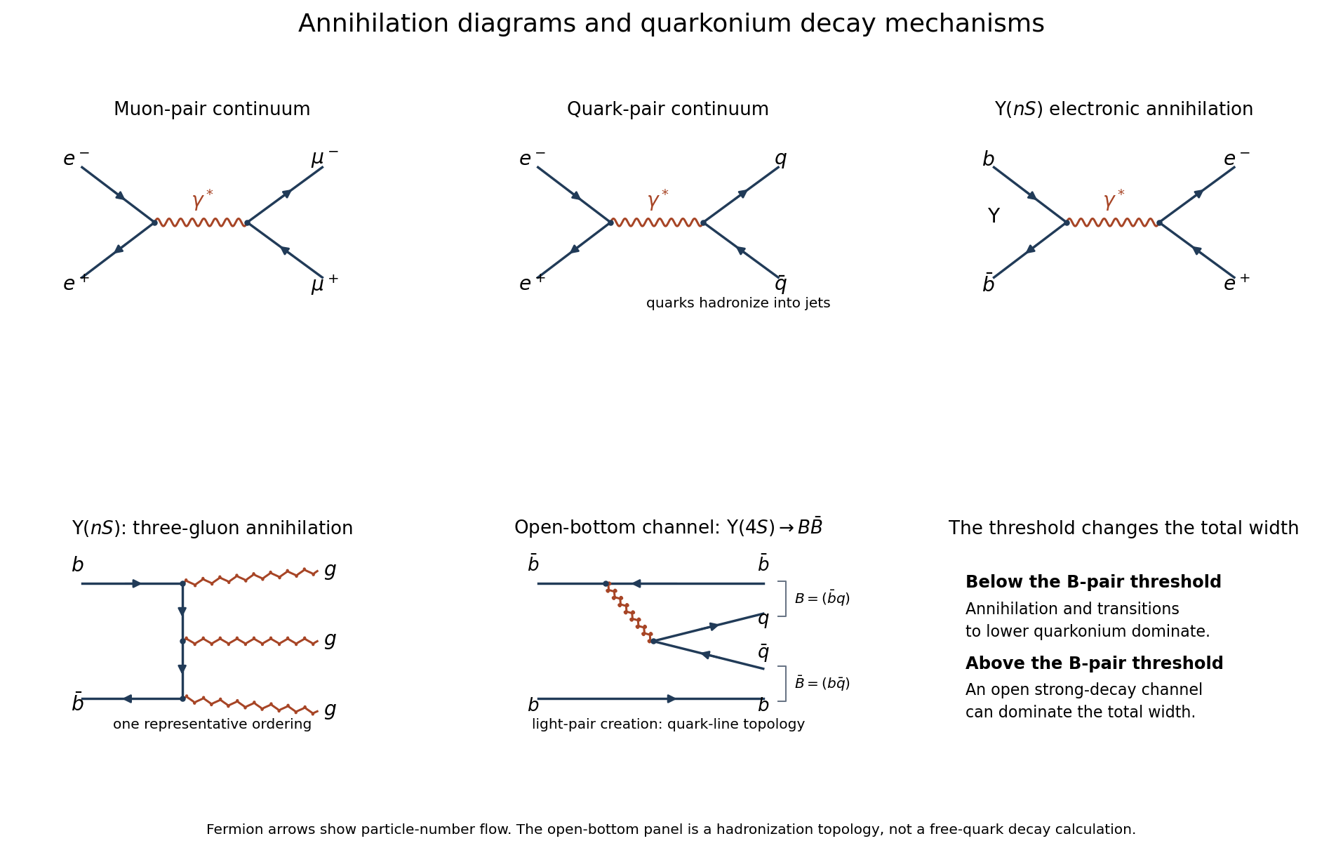
Original Feynman diagrams for electromagnetic pair production, vector-quarkonium annihilation, and the open-bottom decay topology
. Details. 
The Feynman rules give, up to signs and factors of ,The two vertices supply , and the photon propagator supplies . Each external current scales as , so the complete amplitude is of order , and its squared magnitude is of order . The two-body relativistic scattering cross-section supplies the remaining from flux and phase space. Integrating the angular distribution yields . Keeping only the squared propagator while ignoring the external currents would incorrectly predict .
A quark of charge contributes times the massless muon rate. With open and , the hadronic R ratio isThis is the requested massless leading-QED continuum approximation. Strong corrections, physical hadron thresholds, resonance contributions and Z exchange are separate effects; the pure photon formula is not a complete high-energy electroweak cross section throughout the entire stated range.
Efficiency normalization. Read the original PDF plot as a continuum of about and a maximum around at . The supplied conversion constant givesHence near the peak,If multiplies the displayed cross sections, the required scale isHere is the implied detection efficiency under the common-scale assumption. Using continuum readings – gives approximately –, illustrating the graph-reading precision. The nearby open-bottom threshold also limits the precision of the ideal continuum approximation.
Resonance quantum numbers and widths. Direct formation through a single photon requiresThese are the quantum numbers of the electromagnetic current. This concerns single-photon formation; associated production or two-photon reactions need not obey this restriction.
For a Breit-Wigner resonance cross section, subtract the continuum before finding the full width at half maximum. The plotted excess is about , so its half-height occurs at a total displayed cross section near , not . The crossings are roughly and , with a separation around –. ThusFor spin-one formation from unpolarized electrons and positrons, and . With , the peak resonance cross section and branching fractions relation becomesThe corrected excess is . Taking as a representative graph reading givesThus the plot supportsThe width and electronic partial width are estimates from the printed graph under the prescribed Breit-Wigner and efficiency assumptions; these are not precision world-average values. A scale correction changes the peak height and inferred partial width, but not the peak position or width.
Why the lower Upsilon states are narrow. In electromagnetic production and decay of vector quarkonium, every state can annihilate as . The electronic width probes the wavefunction at the origin, . The radial overlaps differ, but the same short-distance annihilation mechanism operates, so electronic widths remain of comparable order.
The hadronic mechanism changes sharply at . The first three Upsilon mesons lie below it and cannot produce an on-shell B-meson pair. Their leading purely strong annihilation channel is , followed by hadronization: a color-singlet pair cannot annihilate to one gluon, and two gluons cannot match its negative charge-conjugation parity. Three-gluon annihilation carries three powers of in the rate and requires quark-antiquark overlap. Electromagnetic annihilation to light quarks and, for excited states, transitions to lower bottomonium plus pions or photons also contribute.
The fourth state lies above the pair threshold and can instead undergo through light-pair creation, keeping the b and anti-b in separate outgoing mesons. The final panel depicts this quark-line topology; it represents a nonperturbative strong decay, not a free on-shell b quark radiating a real gluon. For two pseudoscalar B mesons the pair is in a P wave to give . Although close to threshold, this open strong channel has a much larger rate than the annihilation channels. Consequently a total width of tens of MeV can coexist with an electronic width below a keV; below threshold the total widths are smaller by hundreds or more, while their electronic widths remain of similar order.
Hyperfine estimate. For two spin-half constituents,The meson hyperfine mass splitting therefore raises the vector mass above the pseudoscalar mass. To infer its coefficient from only one measured mass, adopt the intended simple constituent ansatz that the spin-independent baseline is . ThenFor the spin-one partner,The estimate is the same for and with the supplied equal light-quark masses. The splitting is below , so the strong decay is closed. An electromagnetic transition is open and dominates over weak decay:It preserves electric charge, giving the corresponding charged or neutral B meson; the photon energy is approximately , slightly reduced by recoil. Strictly, the statement that the mass merely includes a spin-spin term does not fix : an independent spin-independent binding energy would leave the baseline unknown. The numerical prediction above explicitly uses the additive constituent-mass approximation.
Articles by others on the same topic
There are currently no matching articles.