Past exam of the probability course of the University of Oxford / 2015 (A13764W1, A8)

Source paper: released examination archive, member 2014/T/a13764w1.pdf. The printed cover dates this examination to 23 June 2015. The initial unlettered prompt in Question 3 is indexed as (a), matching the subsequent printed (b) and (c).

The sample maximum has cumulative distribution functionThe product $x^n$ follows from independence of random variables and the continuous uniform distribution of each observation. For every $x<1$, this cumulative distribution function tends to zero; for $x>1$ it equals one. These are exactly the values of the cumulative distribution function of the constant random variable $1$ at its continuity points. Therefore, by the definition of convergence in distribution,At $x=1$ the limiting cumulative distribution function is discontinuous, so the definition does not require checking that point, although $F_{M_n}(1)=1$ also holds.

Put $Z_n=n(1-M_n)$. Its survival function isFor each fixed $z\ge 0$, eventually $n\ge z$, and the exponential limit gives $(1-z/n{)}^n\to e^{-z}$. Thus its cumulative distribution function tends to $0$ for $z<0$ and to $1-e^{-z}$ for $z\ge 0$. This continuous limiting cumulative distribution function identifies the exponential distribution with rate one:This is the exponential endpoint limit of a uniform maximum: the gap from the upper endpoint is typically of order $1/n$, although the maximum itself approaches a constant.

The moment-generating function of a real random variable $X$ isfor real $t$ for which this expected value is finite. Because the integrand is nonnegative, the extended expected value is always defined, but it may equal $+\infty$. We always have $M_X(0)=1$; the usual uniqueness and convergence theorems require finiteness on an open interval containing zero. When this condition holds, derivatives at zero recover the moments, $M_X^{(r)}(0)=\mathbb{E}[X^r]$.

Using the probability mass function of the Poisson distribution and the power series of the exponential function,This moment-generating function of a Poisson distribution is finite for every real $t$. It also covers $\mu =0$, when $X=0$ with probability one and the moment-generating function is identically one.

Complete the square in the integral against the standard normal density:The remaining integral is one because its integrand is the probability density function of the normal distribution $N(t,1)$. Hence the moment-generating function of a standard normal variable is finite on the whole real line.

The Poisson process gives $N_k\sim \mathrm{Pois}(k)$, with expected value and variance both equal to $k$. Consequently $Y_k=(N_k-k)/\sqrt{k}$. Scaling and translating the argument in the moment-generating function of a Poisson distribution gives, for every real $t$,The centering term must remain inside the exponent: omitting it would leave a divergent first-order contribution.

For fixed real $t$, Taylor's theorem for the exponential function givesSubstituting into the previous moment-generating function,The continuity theorem for moment-generating functions states that, if the moment-generating functions of $Z_n$ and $Z$ are finite on a common open interval containing zero and $M_{Z_n}(t)\to M_Z(t)$ throughout that interval, then $Z_n\stackrel{\mathrm{d}}{\to }Z$. Here finiteness holds for all real $t$, and the limit is the moment-generating function of a standard normal variable. ThereforeThis proves the required instance of the Poisson central limit theorem directly from moment-generating functions; no appeal to a general central limit theorem is needed.

Write $A_k=N_{2k}-N_k$ and $B_k=N_k$. The stationary increments and independent increments of the Poisson process make $A_k$ and $B_k$ independent random variables, each with Poisson distribution of parameter $k$. ThusMultiplication of the two moment-generating functions givesThe odd terms cancel in Taylor's theorem, so $\log M_k(t)=t^2+O(k^{-1})$. The limit $e^{t^2}$ is the moment-generating function of a normal distribution with mean zero and variance two. The same continuity theorem for moment-generating functions therefore yieldsIn particular, the two equal-length increments must be separated before using independence: $N_{2k}$ and $N_k$ themselves are dependent.

The joint probability density of the two independent standard normal random variables is $(2\pi {)}^{-1}{e}^{-(x^2+y^2)/2}$. The polar coordinates map has absolute Jacobian determinant $r$, so the change of variables for probability densities givesAt the origin the angle may be assigned arbitrarily: that point has probability zero. The joint probability density factorizes as a Rayleigh distribution density $r{e}^{-r^2/2}$ and a continuous uniform distribution density $1/(2\pi )$. Hence $R$ and $\Theta$ are independent.

For $u>0$, substitute $s=r^2/2$ to findTherefore $R^2\sim \mathrm{Exp}(1/2)$, equivalently ${\chi }_2^2$, and applying a measurable function to $R$ preserves its independence from $\Theta$. Explicitly, with $S=R^2$,Thus $\Theta \sim \mathrm{Unif}[0,2\pi )$ and $S\sim \mathrm{Exp}(1/2)$ independently. This polar decomposition of a planar standard normal vector separates the uniformly distributed direction from its random squared distance.

Set $\alpha =\arctan c\in (0,\pi /2)$. In polar coordinates, the event is $\sin \Theta >c|\cos \Theta |$, the angular sectorBecause $\Theta$ has the continuous uniform distribution on an interval of length $2\pi$, the probability is the sector's angular length divided by $2\pi$:The symmetry of the standard normal distribution in $Y$ makes the lower sector $Y<-c|X|$ equally likely. Their disjoint union is $|Y/X|>c$, apart from $X=0$, an event of probability zero. Therefore the requested cumulative distribution function isThis is the unit-scale half-Cauchy distribution. At $z=0$ there is no atom, and as $z\to \infty$ the cumulative distribution function tends to one.

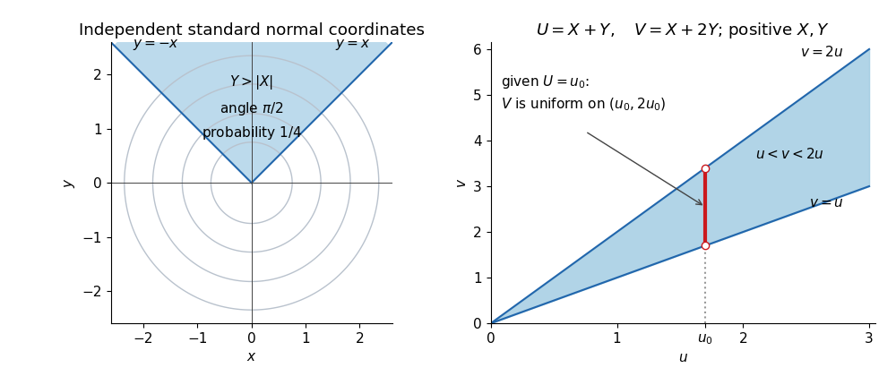
The left panel uses $c=1$, giving a sector of angle $\pi /2$ and probability $1/4$. The right panel displays the domain $u<v<2u$ for the next change of variables for probability densities; a vertical section through it determines the conditional range.

The inverse linear transformation isThe positive support $x>0,y>0$ is exactly $u>0$ and $u<v<2u$. The independence and rate-one exponential distributions give $f_{X,Y}(x,y)=e^{-x-y}$ there. Since $x+y=u$, the change of variables for probability densities yieldsAlthough the density's value depends only on $u$, its support does not factor as a product of fixed intervals. Thus this expression does not imply independence of $U$ and $V$.

Integrating the joint probability density across $u<v<2u$ gives the marginal densityFor every $u>0$, the conditional probability density is consequentlyHenceThis also follows from two independent exponential variables conditioned on their sum: given $X+Y=u$, the variable $Y$ is uniform on $(0,u)$, and $V=u+Y$. Conditioning on $U=u$ here is defined through the conditional probability density, rather than division by $\mathbb{P}(U=u)$, which is zero. The endpoint $u=0$ lies outside the positive marginal support and needs no specified conditional law.

For fixed $v>0$, the support inequalities become $v/2<u<v$. The marginal density is thereforeIt is nonnegative and integrates to $2-1=1$. Another interpretation is that $V=X+2Y$ sums independent exponential random variables of rates $1$ and $1/2$, so it has a hypoexponential distribution. The mean is $1+2=3$, which agrees with ${\int }_0^{\infty }v(e^{-v/2}-e^{-v})dv=4-1=3$.

The strong law of large numbers says that, for real independent and identically distributed random variables $Z_1,Z_2,\dots$ with $\mathbb{E}|Z_1|<\infty$,The assertion is almost sure convergence of the entire sequence of sample means. Finite first absolute moment suffices; a finite variance is not required.

Put $q=1-p$ and ${\xi }_i=Y_i-Y_{i-1}$. The Markov property and the state-independent transition probabilities show that, conditional on the whole previous history, ${\xi }_i$ is $+1$ with probability $p$ and $-1$ with probability $q$. Multiplying these conditional probabilities for any finite step sequence proves that the ${\xi }_i$ are independent and identically distributed random variables, withBecause $Y_n=k+{\sum }_{i=1}^n{\xi }_i$, the strong law of large numbers givesIn particular, $Y_n\to +\infty$ almost surely. This stronger pathwise consequence will determine both eventual crossings and the asymptotic first-passage times.

For $k=0$, the target is reached at time zero, so $h_0=1$. For $k<0$, the preceding almost sure convergence gives $Y_n\to +\infty$ with probability one. A sample path with unit upward and downward steps must visit every intermediate integer when it crosses from a negative value to a positive value. It must therefore visit zero at a finite time. ThusThe unit-step property matters: positive long-run displacement alone would not force a walk with larger upward jumps to land exactly on zero.

The first-step analysis gives $h_0=1$ and, for $k\ge 1$,The minimal nonnegative solution for hitting probabilities theorem states that the probability of ever hitting a target is the pointwise smallest nonnegative solution of this transition recurrence with value one at the target. It follows by comparing any such solution with the probabilities of hitting within $n$ steps, then taking their increasing limit.

The characteristic equation $p{r}^2-r+q=0$ has distinct roots $1$ and $\beta =q/p\in (0,1)$. Hence every solution on the nonnegative integers with boundary value one has the formIf it is nonnegative for all $k$, taking $k\to \infty$ forces $A\ge 0$, and therefore $g_k-{\beta }^k=A(1-{\beta }^k)\ge 0$. The candidate $g_k={\beta }^k$ is itself nonnegative and satisfies the recurrence and boundary value. It is consequently the minimal solution, giving the biased random walk hitting probabilityOn the negative half-line the already established values $h_k=1$ satisfy the same recurrence away from zero. No unproved boundary condition at infinity has been imposed.

Since $Y_n\to +\infty$ almost surely, only finitely many early values can attain the global minimum; it is a finite integer. Also $W\le Y_0=0$. For every nonnegative integer $m$, the unit-step property and translation invariance of the increments giveSubtracting consecutive tails yields the probability mass functionThus $-W$ has the geometric distribution counting failures before the first success, with success parameterThis support convention is essential: the minimum of an upward-biased random walk can equal its starting position, so $-W=0$ has positive probability.

Work on the single event of probability one where $Y_n/n\to \mu =2p-1>0$. On every sample path in that event, $Y_n\to +\infty$ and the unit-step property ensures that every positive integer $j$ is reached, so $T_j<\infty$. Starting from zero requires at least $j$ steps to reach $j$, hence $T_j\ge j$ and $T_j\to \infty$.

The convergent numerical sequence $Y_n/n$ on this fixed sample path also converges along its possibly random subsequence $n=T_j$. Since $Y_{T_j}=j$,Taking the reciprocal is valid because $\mu >0$. We obtainThis is a first-passage law of large numbers for an upward skip-free random walk. No independence between the hitting times and the path is needed: almost sure convergence already supplies convergence along every diverging subsequence on the same event.