Source paper: www.whatdotheyknow.com/request/oxford_physics_past_papers_2/response/2340696/attach/5/Physics%20Papers%202016.pdf?cookie_passthrough=1. The cover identifies Hilary Term 2017, 11 January; the bundle's 2016 filename does not determine the examination year. We use natural units , the mostly-minus Minkowski metric, and Feynman propagators with the prescription.
Treat and as independent variables in the Euler-Lagrange equations. Write , and assume the scalar potential is real and differentiable. Variation with respect to givesConsequently the equations for the complex scalar field and its complex conjugate areNo polynomial assumption is needed: only the first derivative of the scalar potential enters. For , both reduce to the free Klein-Gordon equation.
For a constant real parameter, . The phases therefore cancel separately in the kinetic term and in , leaving any unchanged. This is the global phase symmetry of a complex scalar field, with circle group .
Use infinitesimal variations per unit parameter, , . The Lagrangian density is exactly invariant, so no total-derivative correction is needed in Noether's theorem. The Noether current isIt depends only on derivatives of the Lagrangian density with respect to field derivatives, so the derivative-free scalar potential cannot alter its form. Direct differentiation cancels the mixed first-derivative terms:Thus it is conserved on solutions of the Euler-Lagrange equations. Its spatial integral is a conserved Noether charge when the flux through the boundary vanishes. Its overall sign is fixed here by ; reversing the orientation of the phase transformation reverses the current.
Let . The conjugate momentum fields are and . Inserting the given mode expansion of a free field into produces spatial Dirac delta factors. The and terms vanish after integration: they contain on , and . The number-conserving terms instead add their two frequency factors, cancelling the mode normalization. The un-subtracted ordered expression isThe last term is an infinite vacuum constant, not a finite physical vacuum charge. Choosing the Fock vacuum to have zero Noether charge, equivalently using normal ordering, givesA state containing quanta created by and by has Noether charge . Thus the two families describe opposite unit Noether charges; with this source's current the quantum has positive Noether charge and the quantum negative Noether charge. This is an internal Noether charge; identifying it with electric charge requires a specified electromagnetic coupling. The vacuum subtraction of a complex scalar charge leaves all commutators unchanged.[ref]
Quantum Field Theory by David Tong. Section 2.5, complex scalar fields and their opposite-charge oscillator families; the phase convention fixes the overall sign
Scope of the expansion: a fixed-frequency expansion with time-independent oscillator coefficients is the free-field or asymptotic-field form. For arbitrary interacting , it can be used as canonical oscillator coordinates at a chosen time, rather than as the exact interacting time dependence. For example, gives , which a generic free plane-wave superposition does not satisfy. The Noether charge and its generator action remain valid in the interacting theory; the symmetry does not depend on using a free Hamiltonian.
The two oscillator families commute with each other. Their canonical commutation relations giveBoth terms in the mode expansion of a free field therefore acquire the same factor, givingThe Noether charge is the generator of the internal symmetry. In the active-operator convention , repeated commutators giveThe sign agrees with part b. A negative sign for would correspond to the opposite current convention, not to the current used here. Subtracting a multiple of the identity from to fix the vacuum Noether charge has no effect on this generator relation.
In spacetime dimensions, and a dimensionless action requires . Since , the canonical kinetic term fixes . The cubic and quartic terms then giveThese brackets denote mass dimensions. The cubic coupling is dimensionless at , whereas the quartic coupling is dimensionless at . Hence there is no single dimension in which both nonzero couplings are dimensionless. For example, at the cubic coupling still has mass dimension one.[ref]
Let be the free Feynman propagator, and abbreviate , . Expand the normalized Dyson series, so vacuum bubbles cancel between numerator and denominator, and retain the connected correlation function. Wick's theorem yieldsThese are respectively the free line, the quartic tadpole diagram, the two-cubic-vertex bubble diagram, and an tadpole contribution to a cubic-theory two-point function, attached by a bridge to the vertex carrying both external legs. The last graph is connected but is a one-particle-reducible Feynman diagram; removing its bridge disconnects it. It must be included when all connected graphs are requested. It disappears if an additional vanishing-one-point-function renormalization condition and its corresponding tadpole subtraction are imposed; that convention was not specified here.
The factors can be counted directly. The quartic term has attachments for the two labelled external legs, divided by . At second order in the cubic interaction the expansion denominator is . There are 36 Wick contractions for the bubble, and 36 for the attached-tadpole graph, giving for each. Thus each loop topology shown has symmetry factor . Disconnected products of one-point functions and vacuum bubbles are not part of .[ref]
Quantum Field Theory by David Tong. Sections 3.3–3.4, Wick contractions and diagrammatic perturbation theory
The one-loop cubic-quartic scalar vertex classification follows without truncating arbitrarily in powers of the couplings. A connected graph with external legs, cubic vertices, quartic vertices and loop number satisfiesFor , the only possibilities are or , exactly those just listed.
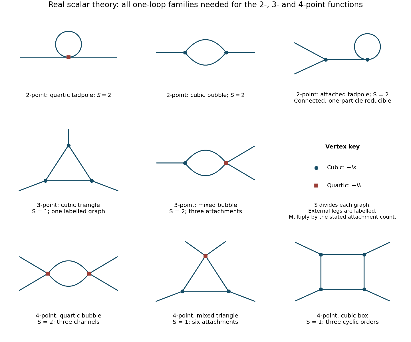
One-loop Feynman diagrams in the real cubic-plus-quartic scalar field theory, with symmetry factors and channel multiplicities
. Details. 
For the amputated one-particle-irreducible vertex, every internal bridge is forbidden. Define the Feynman integralsFor , the counting identity in part b gives . The only one-particle-irreducible Feynman diagrams are a triangle of three cubic vertices and a two-propagator bubble joining one cubic and one quartic vertex. Write for the amputated Feynman vertex, including its overall factor of . With all external momenta incoming,The triangle has for labelled external legs. The mixed bubble has because its two internal lines may be interchanged. There are three distinct terms, according to which external leg is attached to the cubic vertex; the other two attach to the quartic vertex. No tadpole attached by a bridge is one-particle irreducible.
The requested position-space three-point correlation function is obtained by restoring the external propagators and a Fourier transform:The tree-level contribution would replace the last factor by . This explicitly distinguishes the amputated vertex from the correlation function while giving all loop integrations in momentum space.
Let denote the amputated Feynman vertex, with tree term . A one-loop one-particle-irreducible Feynman diagram has , allowing three families: two quartic vertices, two cubic vertices and one quartic vertex, or four cubic vertices. DefineUsing from part c and writing , the complete one-loop result isIn each term of the middle sum, are the two complementary indices. Their order does not change the integral after a loop-momentum redefinition.
The first line contains three bubble channels, one for each partition of the four labelled external legs into two pairs. Each has from interchanging its two identical internal lines. In the second line, the quartic vertex carries a chosen pair of external legs, giving mixed triangles. Each has . In the last line, cyclic orderings of four labelled external legs are identified under rotation and reversal, leaving boxes, again with each. The figure in part b shows one representative of each family and its multiplicity. External-leg corrections and tadpoles connected by bridges are excluded because is a one-particle-irreducible vertex. All integrals are left unevaluated, as appropriate here.
A free contraction must connect one and one field. In momentum space,Represent the nonzero propagator by a directed line so the two conjugate ends remain distinguishable; an undirected line alone would incorrectly allow same-charge contractions. Choose one consistent arrow convention, for example pointing from the starred end to the unstarred end.
The interaction contains two identical fields and two identical fields. Their assignments cancel the coefficient , givingThe vertex has two incoming and two outgoing arrows. Include at every vertex, integrate for each independent loop, and divide by the oriented graph's symmetry factor. There is no fermion-loop sign.
The two real fields have canonical normalization becauseThereforeThe interaction is invariant under rotations and reflections of . The continuous rotations are the original complex-field symmetry. The factor follows from both the original and the square of the in .
The propagator carries a real-species label rather than a charge-flow arrow:Differentiating the interaction with respect to its four external real fields gives the compact tensor ruleThus four legs or four legs give , while two of each give . Vertices with an odd number of either species vanish. For example, , whereas . These factors already account for assignments at one vertex; graph symmetry factors must still be included separately. Momentum conservation and loop measures are the same as in part a.
Use renormalized propagators of mass and tree vertex . The interaction counterterms have Feynman factors for a two-leg mass insertion and for a four-leg insertion. At one loop the two-point one-particle-irreducible vertex isThe directed tadpole has : interchanging its two ends would reverse the field labels, so the real-scalar tadpole's factor does not apply. It is independent of external momentum, so no wave-function counterterm is required at this order.
For the four-point vertex, label the two unstarred incoming fields by and the starred ones by , with all momenta incoming. The tree contact, the three oriented bubbles and the contact counterterm giveThe first bubble has two equivalent arrows along the same direction between its vertices, giving . In the other two channels the arrows oppose one another, and interchanging the lines does not preserve their oriented attachments, giving . This is the oriented complex-scalar quartic graph factors rule.
The mass tadpole is order , while the four-point loop is order . In the multiplicative coupling convention of the source,The distinction between and the whole additive four-leg coefficient matters for the requested order counting.
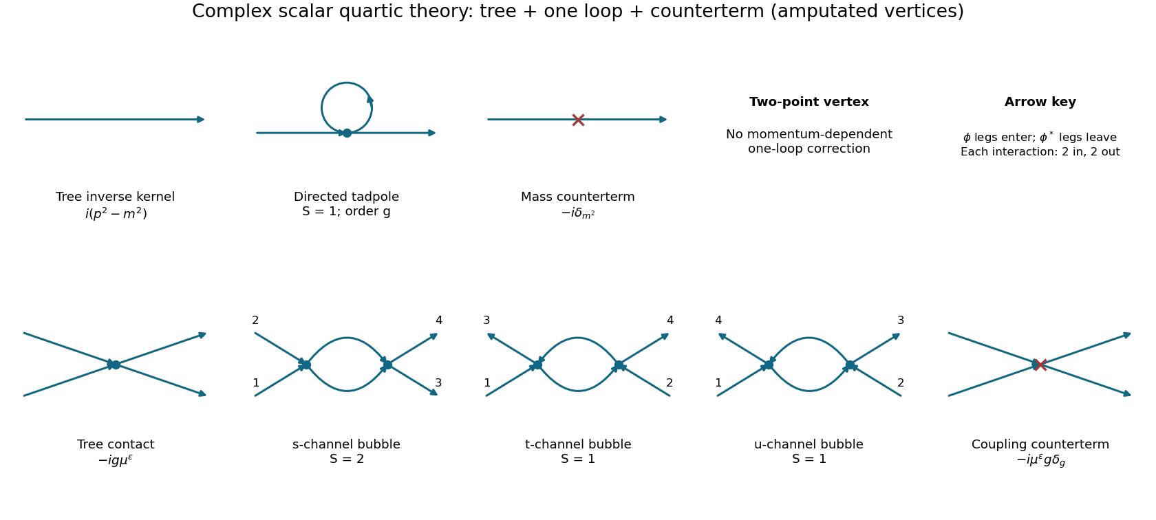
Tree, loop and counterterm contributions to the two-point and four-point vertices of a complex scalar field
. Details. 
Source correction: equation 11 on the original page has . The dimensionally regulated integral instead contains . This is not an interchangeable convention: for and , the correct factor has a logarithmic ultraviolet pole, whereas the printed is finite.
To obtain the correct expression, shift the loop momentum and perform a Wick rotation. For positive Euclidean , introduce a Schwinger parameterization:The derivation first holds in the convergent range and defines the result elsewhere by analytic continuation. For integer , rotating back giveswith the branch inherited from . This is the Lorentzian continuation of the Euclidean massive loop integral.
Set , , . Since ,Consequently the directed tadpole in part d givesThe counterterm is , so cancelling only the pole in the minimal subtraction scheme requiresThis is the quartic complex-scalar mass renormalization result. The scale factors and logarithms contribute finite terms at this order and do not change the displayed pole coefficient. A real-field check gives a tadpole coefficient , in agreement with the oriented complex-field computation.
To first order, invert and use :The remainder is a perturbative statement at fixed regulator. When differentiating, hold the bare mass fixed as well as ; otherwise the mass running would not be defined by a fixed bare theory. Since ,Thus, with the source's extra factor of one half,The factor from the running dimensionless bare coupling cancels the counterterm pole. Differentiating as though were independent of would miss this finite result. Some conventions call itself the mass anomalous dimension; that convention is twice the one defined here.
At fixed external momenta, fixed regulator and fixed bare coupling, define the total scale derivativeThe bare vertex has no independent dependence on the arbitrary renormalization scale. Differentiating therefore givesDefining the two scale-response functions as in the source yieldsThis is the Callan-Symanzik equation. Its minus sign and factor follow from the specified multiplying the bare vertex. In particular, the source's is twice the field anomalous dimension defined using . A convention change must be made consistently in both definitions and equation.
The dimensionless bare parameter is , so direct differentiation at fixed givesThe dimensionful bare vertex itself is scale independent. Reexpressing it as introduces only the combination . HenceThere is no multiplicative field rescaling in this bare parametrization, soThis does not assert that the interacting renormalized field has zero anomalous dimension. It says that the unrescaled bare field has no additional normalization factor under this change of the arbitrary scale.
Write . Allow a general bare coefficient temporarily, so the starting equation is . Substitute and apply the product and chain rules:Multiplying by identifiesThus the renormalization-group beta function transforms by the chain rule under a coupling reparametrization, while the field coefficient also records the scale dependence of the finite or divergent field normalization. For the actual bare parametrization here, substitute and .
At fixed regulator abbreviateThe coupling expansion is , whose inverse is . Using part c before removing the regulator,Therefore the regulator-free coefficients at the orders determined by the supplied expansions areThe canonical term vanishes, and the factors of cancel the simple poles. The finite coefficients and higher positive powers of do not enter these leading regulator-free terms. Inverting the coupling is essential: substituting too early would incorrectly give .
The calculation establishes finiteness only at the displayed perturbative orders. Higher-order pole cancellations require the higher-order coefficients, as the next part makes explicit.
Retain the specified leading poles and write , . Solving recursively givesThe scale derivative must again be reexpressed in the renormalized coupling:The leading-pole consistency under coupling reparametrization shows that a finite renormalization-group beta function requires the two-loop double-pole consistency conditionThe leading two-loop pole is fixed by the one-loop simple pole; it is not an independent parameter. This is an instance of the simple-pole formulas for minimal-subtraction renormalization group functions and their higher-pole consistency relations.
The source's leading-pole truncation does not fix the finite two-loop coefficient of the beta function. For example, adding the omitted term leaves the double-pole condition unchanged but contributes to the finite beta function. Thus cancelling the displayed term is not a claim that the physical two-loop running vanishes.
Articles by others on the same topic
There are currently no matching articles.