Past exam of the theoretical physics II course of the University of Cambridge / 2019

The Heisenberg equation of motion and the spin commutation relations give, componentwise,Thus $\boxed{d\mathbf{S}/dt=\gamma \mathbf{S}\times \mathbf{B}}$. For constant magnetic field this is Larmor precession: the component along $\mathbf{B}$ is conserved and the transverse components rotate. In particular, for $\mathbf{B}=B\hat{\mathbf{z}}$,The signed angular velocity is $-\gamma \mathbf{B}$; the positive precession rate is $|\gamma B|$.

Here the dimensionless spin one-half operator is $S_x={\sigma }_x/2$. Since the Pauli matrix obeys ${\sigma }_x^2=I$, the even and odd terms of the matrix exponential giveThis is the exponential of a Pauli vector for an $x$-axis rotation. With a physical spin angular momentum $S_x^{\mathrm{phys}}=\hslash {\sigma }_x/2$, the exponent is $-i\theta S_x^{\mathrm{phys}}/\hslash$.

Use the ordered orthonormal basis $(|1s⟩,|2p_x⟩)$. The projected Hamiltonian between pulses is $H_0=-\Delta {\sigma }_z$, so its free time-evolution operator through a period isAcross one instantaneous pulse, integrating the Schrödinger equation givesusing the exponential of a Pauli vector. The finite free Hamiltonian contributes vanishing evolution during the zero-duration kick. A period measured immediately before successive pulses therefore consists of the kick followed by free evolution. Composition givesThis is the Floquet operator at the specified phase of the pulse train. Actual hydrogenic energy levels are not opposite numbers: the displayed convention subtracts their midpoint, with $\Delta =(E_{2p}-E_{1s})/2$. Restoring that midpoint multiplies the result by an unobservable global phase. Likewise $E$ in the given Hamiltonian denotes the electric coupling per unit length; if it is instead a physical electric-field strength, its charge factor must be included in $E{x}_0$.

Put $\alpha =\Delta \tau /\hslash$ and $\beta =E{x}_0\tau /\hslash$. The Pauli matrix multiplication law gives the pulse-and-precession spin one-half mapBecause $C^2+|\mathbf{v}{|}^2=1$, a suitable angle and unit vector for the rotation areIf the denominator vanishes, $U=\pm I$ and the axis is arbitrary. The Bloch vector $\mathbf{r}=⟨\mathbf{\sigma }⟩$ rotates through $\theta$ about $\mathbf{n}$ per period; after $N$ periods the angle is $N\theta$. The eigenphases equivalently give quasienergies $\pm \hslash \theta /(2\tau )$ modulo $2\pi \hslash /\tau$.

In the two-orbital subspace the position operator is $X=x_0{\sigma }_x$. The Heisenberg equation of motion between pulses gives $P/m=(i/\hslash )[H_0,X]=(2\Delta x_0/\hslash ){\sigma }_y$, henceThus two components of the Bloch vector directly describe the mean position and momentum; its third gives the orbital population imbalance. The electric kick rotates about the position axis, leaving $⟨X⟩$ unchanged at the kick, while free evolution mixes the position and momentum components. Starting in $|1s⟩$, one complete period giveswhich exhibits the induced motion explicitly. These are projected two-orbital observables.

Assume a real, central, short-range potential and elastic quantum scattering. At large radius, normalize the stationary wavefunction aswhere $k=\sqrt{2mE}/\hslash$ and $\theta$ is the scattering angle. Equal incoming and outgoing speeds give the differential scattering cross-section $d\sigma /d\Omega =|f(\theta ){|}^2$.

The partial-wave scattering expansion separates the spherical harmonics. The incident plane wave has expansion ${\sum }_{\ell \ge 0}{i}^{\ell }(2\ell +1)j_{\ell }(kr)P_{\ell }(\cos \theta )$, with Spherical Bessel functions $j_{\ell }$ and Legendre polynomials $P_{\ell }$. The regular radial solution outside the potential has asymptotic form $u_{\ell }\propto \sin (kr-\ell \pi /2+{\delta }_{\ell })$. Its real scattering phase shift ${\delta }_{\ell }$ changes the ratio of outgoing to incoming waves to the Partial-wave S-matrix $S_{\ell }=e^{2i{\delta }_{\ell }}$. Matching outgoing coefficients yieldsHere $\ell$ labels the orbital angular momentum, with squared magnitude ${\hslash }^2\ell (\ell +1)$. The assumption of purely elastic scattering is what makes every $S_{\ell }$ have unit modulus.

Integrate the squared partial-wave expansion of a scattering amplitude over the solid angle. Legendre polynomial orthogonality eliminates terms with unequal angular-momentum indices, givingAt zero scattering angle, $P_{\ell }(1)=1$ and $\mathrm{Im}(e^{i{\delta }_{\ell }}\sin {\delta }_{\ell })={\sin }^2{\delta }_{\ell }$. ConsequentlyThis is the optical theorem. In the present elastic problem the total and elastic cross sections coincide. For an absorptive interaction the inclusive total still obeys the optical theorem, but need not equal the integral of the elastic differential cross section.

The radial S wave vanishes at the hard surface, so outside the sphere $u_0(r)=A\sin [k(r-R)]$. Comparison with $A\sin (kr+{\delta }_0)$ givesThe hard-sphere S-wave scattering amplitude and cross section are thereforeThe three prominent features are the finite low-energy limit ${\sigma }_0\to 4\pi R^2$, the oscillations with exact zeros at $x=n\pi$ for positive integers $n$, and the decreasing envelope ${\sigma }_0\le 4\pi /k^2$. The zero-energy value is four times the geometric area $\pi R^2$. Near zero the normalized cross section is $1-x^2/3+O(x^4)$. The large-$k$ fall here concerns the S wave alone; summing all partial waves gives a different high-energy total.

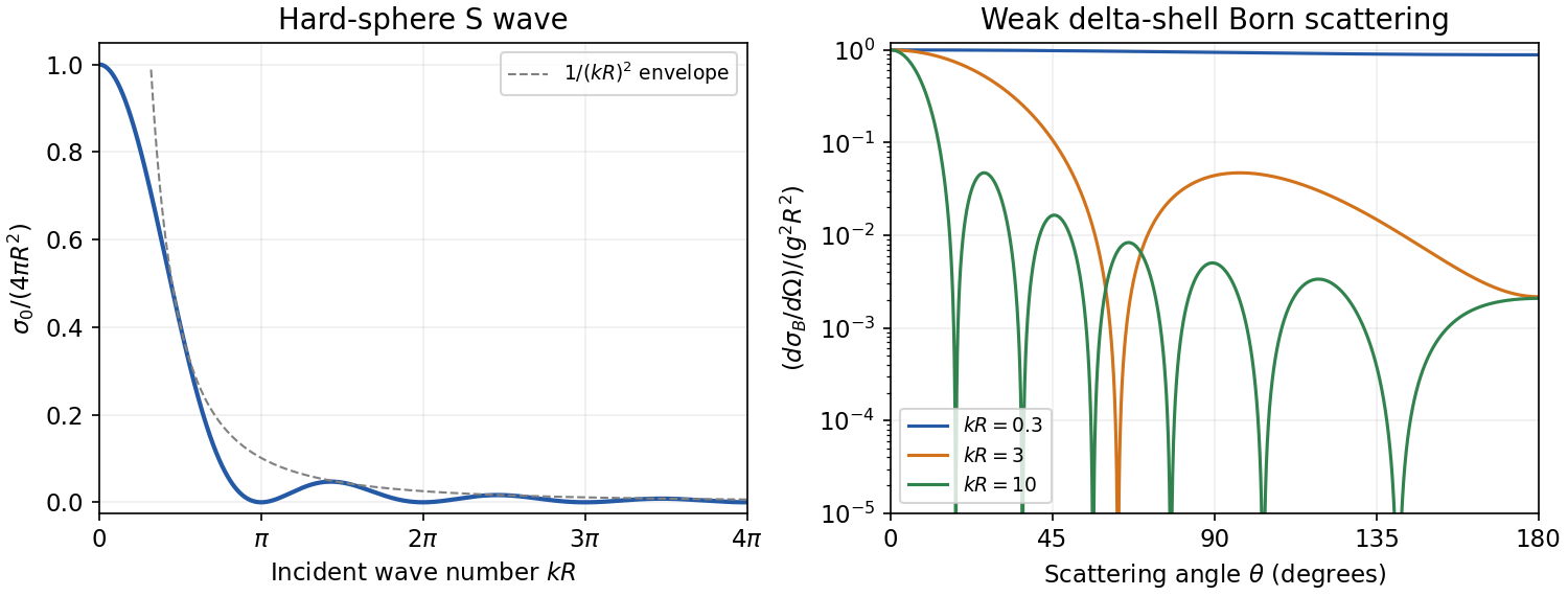
In the first Born approximation, let $q=|{\mathbf{k}}^{\prime }-\mathbf{k}|=2k\sin (\theta /2)$ be the transferred wave number. The angular integral in the three-dimensional Fourier transform is $4\pi \sin (qr)/(qr)$, soWriting $g=2m{V}_{0}R/{\hslash }^2$ and $\mathrm{sinc}u=\sin u/u$, with value one at zero, the delta-shell Born amplitude givesFor $kR\ll 1$ the scattering is approximately isotropic, with total cross section $4\pi g^2{R}^2$. For $kR\gg 1$ it has a forward lobe of angular width of order $(kR{)}^{-1}$ and oscillatory zeros where $2kR\sin (\theta /2)=n\pi$. At a fixed nonzero scattering angle, its envelope decreases as $k^{-2}$. The right-hand panel of the figure shows this angular dependence.

For real $V_0$ the first-order scattering amplitude is real, so inserting it literally in the optical theorem would predict zero total cross section, contrary to its nonzero squared modulus. The first Born amplitude alone does not satisfy the optical theorem at order $V_0^2$. This is an order-of-approximation issue: the squared first-order amplitude is already second order, and the second Born term supplies the required second-order imaginary forward amplitude. At first order both sides vanish. A weak-shell regime is needed for the Born truncation itself to be accurate.

For bosonic creation operators and bosonic annihilation operators, the canonical commutation relations areFor fermionic annihilation operators and their adjoints, the canonical anticommutation relations areThe respective number operators are $n_i=a_i^{†}{a}_i$ and $n_i=f_i^{†}{f}_i$. Their allowed eigenvalues are $\boxed{0,1,2,\dots \text{ for bosons};0,1\text{ for fermions}}$. In the fermionic case $n_i^2=n_i$, so its eigenvalues must satisfy $n^2=n$; this is the single-mode Pauli exclusion principle.

In the ordered product basis $(|\uparrow \uparrow ⟩,|\uparrow \downarrow ⟩,|\downarrow \uparrow ⟩,|\downarrow \downarrow ⟩)$, the two-spin XY Hamiltonian isThe transverse term exchanges opposite spins and leaves parallel spins unchanged. Diagonalizing its two-dimensional block gives the complete orthonormal eigenbasisThe antisymmetric state is the singlet state; the other three are triplet states. Accidental equality of energies does not invalidate this eigenbasis.

There is a normalization mismatch in the printed definitions: ${\sigma }^x\pm i{\sigma }^y$ have nonzero entries of magnitude two, whereas a single fermionic creation or annihilation operator has magnitude one. To obtain the intended Jordan–Wigner transformation, use normalized spin ladders $s_j^{\pm }=({\sigma }_j^x\pm i{\sigma }_j^y)/2$. The given fermion expressions represent these $s_j^{\pm }$. The two-site Jordan-Wigner normalization and signs then fix every factor unambiguously.

Put $n_j=f_j^{†}{f}_j$ and $P_1=e^{i\pi n_1}=1-2n_1$. The canonical anticommutation relations give $P_1^2=I$, $P_1{f}_1=-f_1{P}_1$, and $[P_1,f_2]=[P_1,f_2^{†}]=0$. HenceandThese are the spin commutation relations, with distinct sites commuting. If one retains the unscaled symbols ${\sigma }_j^{\pm }=2s_j^{\pm }$, the first and last displayed commutators instead equal $-4{\sigma }_j^z$; the off-site commutators remain zero. Setting the unscaled ${\sigma }_j^{-}$ equal to $f_j$ would contradict the original Pauli matrices.

Using the consistently normalized Jordan–Wigner transformation from part (c), write ${\sigma }_1^x{\sigma }_2^x+{\sigma }_1^y{\sigma }_2^y=2(s_1^{+}{s}_2^{-}+s_1^{-}{s}_2^{+})$. Since $f_1^{†}{P}_1=f_1^{†}$ and $f_1{P}_1=-f_1$, the parity string givesThereforeThe orthogonal transformation $b=(f_1+f_2)/\sqrt{2}$, $c=(f_1-f_2)/\sqrt{2}$ preserves the canonical anticommutation relations and diagonalizes this bilinear Hamiltonian:The Fock vacuum is $|\downarrow \downarrow ⟩$, with energy $2h$. Occupying $b$ alone gives the symmetric opposite-spin state with energy $-2J$; occupying $c$ alone gives the antisymmetric state with energy $2J$; occupying both gives $|\uparrow \uparrow ⟩$, up to a global phase, with energy $-2h$. This reproduces the entire spectrum in part (b).

A quantum state ensemble of normalized states $|{\psi }_i⟩$, with probabilities $p_i\ge 0$ and ${\sum }_i{p}_i=1$, has density operatorIt is a positive semidefinite Hermitian operator with trace one, and the Born rule assigns a measurement outcome with projector $\Pi$ the probability $\mathrm{Tr}(\rho \Pi )$.

A pure state has $\rho =|\psi ⟩⟨\psi |$, hence ${\rho }^2=\rho$ and purity of a density operator $\mathrm{Tr}({\rho }^2)=1$. Its only nonzero eigenvalue is one. A mixed state has at least two nonzero eigenvalues and $\mathrm{Tr}({\rho }^2)<1$. The spectral theorem proves the converse criteria, since the nonnegative eigenvalues sum to one. Different quantum state ensembles may give the same density operator; the mere presence of several terms in a preparation list does not make the state mixed if all positive-weight terms represent the same quantum state ray.

Taking the outer product for A and averaging the two orthogonal projections for B givesThe off-diagonal entries in ${\rho }_A$ retain quantum coherence between the $z$-basis states. They are absent from B's classical quantum state ensemble. In particular, $\mathrm{Tr}{\rho }_A^2=1$ and $\mathrm{Tr}{\rho }_B^2=1/2$: A is a pure state, B a mixed state.

The projective measurement probabilities are $P({\sigma }_j=\pm 1)=\mathrm{Tr}[\rho (I\pm {\sigma }_j)/2]$. Both density operators have zero $z$-component of their Bloch vector, soTheir full ${\sigma }_z$ outcome distributions, not merely their mean values, coincide. Along $x$, however,Thus repeated spin measurement along $x$ distinguishes the preparations statistically. A single negative outcome excludes A, while a single positive outcome is compatible with either; under B the probability of $N$ independent positive outcomes is $2^{-N}$.

The opposite $x$-axis pure states have projectors $(I\pm {\sigma }_x)/2$. Averaging them givesTherefore C and B cannot be distinguished by any measurement on the atoms alone. Every POVM outcome has the same probability $\mathrm{Tr}(E\rho )$ for the two preparations; this is the operational equivalence of different quantum state ensembles. Accessible preparation labels or additional correlations would be extra information. C can be distinguished from A by the $x$-axis spin measurement in part (c).

The normalized singlet state has column vector $(0,1,-1,0{)}^{\mathsf{T}}/\sqrt{2}$ in the specified product basis. Its outer product isIt obeys ${\rho }_D^2={\rho }_D$ and has eigenvalues $(1,0,0,0)$, hence purity of a density operator one. The joint two-atom system is therefore a pure state, even though the quantum entanglement prevents assigning a separate pure spin state to each atom.

Taking the partial trace over the left atom in the singlet state gives the right-hand reduced density matrixThus every measurement on the right stream alone has the same statistics as B or C. The joint pure state is compatible with locally mixed states; the correlations reside in the full density operator.

The reduced density matrix has two eigenvalues equal to $1/2$. Its Von Neumann entropy, which is the entanglement entropy of the bipartite pure state, isThis is one bit when base-two logarithms are used. It is the maximum entanglement entropy for a pair of two-dimensional systems, while the joint Von Neumann entropy of the singlet state remains zero.

Take the two magnetic moments along $z$ to be $\pm \mu$, so $H=-\mu B_z{\sigma }_z$ and the two energies are $\mp \mu B_z$. The quantum Gibbs state at inverse temperature $\beta =1/(k_{B}T)$ isIts Bloch vector is $(0,0,\tanh \beta \mu B_z)$. At $B_z=0$, or in the high-temperature limit, it approaches $I/2$; at $T\to 0^{+}$ with nonzero $\mu B_z$, it approaches the lower-energy pure state. Here $\mu$ is the magnitude or signed coefficient multiplying ${\sigma }_z$ in the magnetic Hamiltonian, rather than a moment with an additional unstated factor of two.