Original solutions to the paper released at the source request. The complete editable transcription is retained in the private examination archive.
The iteration of a map is . For every , , so and . A cobweb alternates vertical steps to the graph and horizontal steps to the diagonal, approaching the origin monotonically.
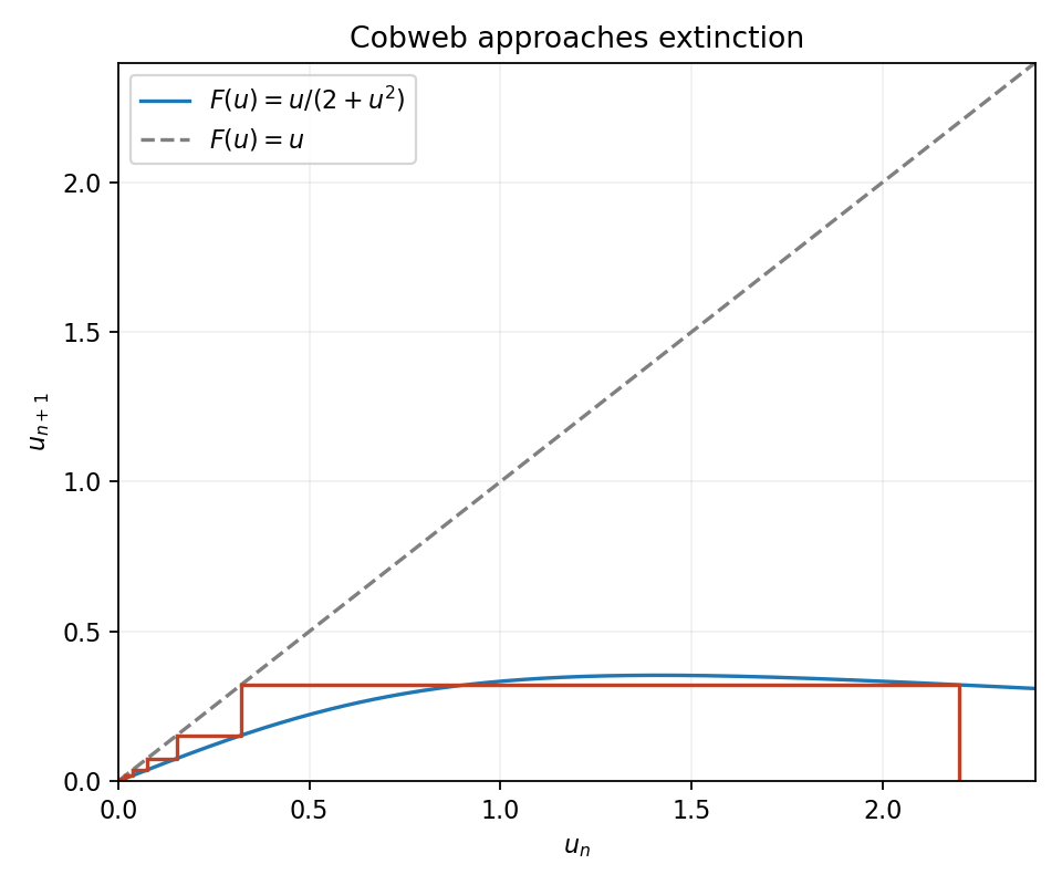
More precisely . The product has a finite strictly positive limit because . Thus for a positive constant depending on the initial biological population.
A positive fixed point requires , so it exists exactly when and is . Differentiating the map at it givesFor and , this fixed-point multiplier is strictly between and . Hence the positive fixed point is linearly asymptotically stable, including ; positivity of makes the lower bound strict.
The fixed-point multiplier decreases continuously with and first reaches the unit circle at . Solving givesIt is stable for and unstable for . At the critical value linear stability is inconclusive. The crossing at is the local signature of a period-doubling bifurcation, rather than a crossing through .
At low density the per-generation growth factor is approximately . The power controls how sharply crowding reduces recruitment or survival when resources become limiting; at high density . Larger therefore means a stronger overcompensation in a population model.
The flip threshold says that sufficiently strong density feedback can destabilize a constant positive biological population and create alternating generations, under the usual nondegeneracy conditions. A local loss of fixed-point stability alone does not establish chaos, nor does it prove every ecological system with stronger crowding must follow the same route.
A fixed point of is also a fixed point of . By the chain rule,If the original fixed-point multiplier has modulus greater than one, its square also exceeds one, so the same fixed point is unstable for the twice-iterated map. New stable fixed points of the twice-iterated map, if present, must be different points; they can represent a genuine two-cycle of the original map.
Law of mass action assigns net substrate gain to autocatalytic replication, substrate-enzyme binding flux , dissociation flux and product-formation flux . ThereforeComplex breakdown to product restores free enzyme but does not restore substrate. Product concentration, if required, satisfies .
Adding the last two equations gives . The initial conditions therefore imply , or . Substitute this in the first two balances:The enzyme inventory is conserved even while substrate can grow autocatalytically.
Use , and slow time . Dividing the equations by their respective concentration and time scales givesThus and . Notice that and the physical enzyme fraction satisfies . The initial values are , for this particular normalization; the threshold analysis compares different initial substrate abundances using a fixed reference scale.
At equilibrium and adding gives . The positive equilibrium isThis condition also gives . The nullclines are and . The second lies above the first for and below it for . Below the first nullcline ; above it . Below the second nullcline ; above it .
At the origin the Jacobian has trace and determinant . Its off-diagonal entries are positive, making the eigenvalues real, so this is an attracting node. At the positive equilibrium the slow reduced derivative is , while the fast derivative is ; equivalently the full Jacobian determinant is negative. Thus the positive point is a saddle equilibrium. Its stable manifold separates extinction from unbounded substrate growth.
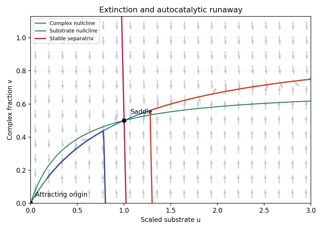
Autocatalytic enzyme phase plane: a fast complex fraction and a saddle threshold separate extinction from substrate runaway
. Details. After an initial layer of duration in slow time, while changes only slightly. The reduced substrate equation isBelow it decreases to zero; above it increases without bound. The exact threshold for initial is the intersection of the saddle equilibrium's stable manifold with that axis. For small it isIn dimensional initial-substrate units the leading threshold is . Comparing the actual initial value to this threshold determines its fate; the reference scale can be held fixed when varying the initial concentration.
The initial sequestration produces an correction if desired. Write the stable manifold as . The invariance equation at leading order gives and . Hencefor fixed parameters away from degenerate limits. The positive correction reflects the substrate consumed in building complexes from the initially enzyme-free-complex state.
The physical strip , is invariant, and the off-diagonal derivatives are nonnegative there, so ordered initial substrate values remain ordered. There are only the attracting origin and the saddle equilibrium. With Dulac function , the divergence of the weighted vector field is , excluding periodic orbits in its interior. The saddle equilibrium separatrix therefore gives the unique threshold on the initial axis: below it solutions tend to extinction, at it they tend to the saddle equilibrium, and above it they escape to infinity. Growth is at most exponential, so this is as time tends to infinity, not a finite-time blowup. This is autocatalytic enzyme clearance with a saddle threshold.
The travelling coordinate has , . Therefore the profile equation isThe wave moves right with speed . It joins a populated equilibrium behind to an empty equilibrium ahead.
The phase-plane equations are , . Nonnegative equilibria require and , hence only . At the origin , so the linear eigenvalues solveFor the roots are complex with negative real part, giving a stable focus. For both are negative real numbers, giving a stable node. Equality is the repeated-root threshold and is not covered by either strict classification.
A nonconstant trajectory approaching a stable focus winds around it infinitely often. Its coordinate therefore changes sign repeatedly near zero. Since the biological population profile must remain nonnegative, such a trajectory cannot represent the wave. The only nonnegative trajectory avoiding that winding at the origin would be the equilibrium itself, which cannot join the populated state. Thus .
On with ,Thus . Since , comparing slopes alone can reverse one's intuition about crossing direction. More directly, for the inward test isso the sloping edge also points into .
The top edge points down by (a), the sloping edge points upward in the inward normal sense by (b), and on the velocity points left. At the region contains only the equilibrium . Thus the closed triangle is forward invariant.
The given unstable saddle equilibrium branch enters its interior from and stays in this compact region. Along it , so decreases and has a limit. An interior limiting orbit with would keep changing , while an interior point with , has and is not an equilibrium. Hence the only possible forward limit is . Ordinary-differential-equation uniqueness prevents reaching and leaving an equilibrium in finite profile coordinate. The whole orbit therefore joins at to at with and .
Consequently . This proves the requested strict-speed result without claiming an unproved conclusion at the repeated-root threshold. It is a trapping triangle for a saturating monostable invasion front.
The reaction Jacobian isIts trace is and determinant is , so both eigenvalues have negative real parts. Explicitly they are . Therefore the homogeneous reaction equilibrium is a stable focus in the absence of diffusion.
The cosine modes satisfy both zero-flux endpoint conditions and . Linearizing the reaction terms gives and . Cancelling the common mode factor yieldsThe derivatives are exactly the entries of the matrix computed in (ii). The zero mode reproduces the stable homogeneous perturbation; positive integers give the possible spatial instabilities.
Put . The mode matrix has trace , so a growing eigenvalue occurs exactly when its determinant is negative:This upward quadratic has two positive roots only if and . Within this isFor such , defineThe unstable modes satisfy . These are strict inequalities: at either endpoint the leading eigenvalue is zero rather than positive.
If , both nonconstant coefficients of are nonnegative, so it is positive for . If , its discriminant is negative, so it is again strictly positive. Therefore .
At the double root can only give a neutral zero eigenvalue if it coincides with an allowed spatial mode; it still gives no positive growth rate. This is the finite-wavenumber onset of a Turing instability, not an oscillatory crossing since the mode trace stays negative.
Small makes every nonzero large, placing them above the finite instability band, where diffusion dominates reaction. The homogeneous zero mode is already stable.
For , the first possible band entry as increases is crossing . Hence the critical length isAt equality the mode is neutral; it is unstable just above this value, while . Thus strictly positive growth has infimum , with no attained smallest length if “unstable” means . The conventional threshold answer is . Larger modes cannot enter earlier because their first-entry lengths are .
A saddle-node bifurcation creates or destroys two equilibria when a real eigenvalue passes through zero with a nonzero quadratic normal-form term. With a parameter orientation chosen so the pair appears for , useThere are no equilibria for , a double nonhyperbolic equilibrium at zero, and equilibria for . The positive branch is stable and the negative branch unstable in the active direction; additional hyperbolic directions can make them a node and a saddle equilibrium. “Supercritical” for a fold depends on this chosen parameter orientation; unlike the pitchfork and Hopf cases it is not an intrinsic distinction between the stability of two possible cubic branches.
The supercritical pitchfork normal form of a dynamical system isThe symmetric equilibrium is stable for and unstable for . Two new stable equilibria emerge on the unstable side of the original branch. Reflection symmetry preserves the pair. The new equilibria approach zero continuously as the parameter reaches the threshold.
A Hopf bifurcation occurs when a simple pair of complex conjugate eigenvalues crosses the imaginary axis at nonzero frequency. A supercritical normal form of a dynamical system isWriting gives and . A stable periodic orbit of radius is born for as the equilibrium loses stability. In contrast, a subcritical Hopf has an unstable small periodic orbit on the side where the equilibrium is still stable.
The Lorenz equilibria satisfy , and . ThusAt the origin the third eigenvalue is and the other two solve . Hence the origin is stable for , has one zero eigenvalue at , and becomes a saddle equilibrium with one unstable direction for . The symmetry interchanges the new branches.
The nonzero-equilibrium characteristic polynomial isNear its Routh-Hurwitz inequalities are strict, so both new branches are stable. More explicitly, center-manifold projection at givesThe linear coefficient crosses positively and the cubic coefficient is negative. Therefore the equilibrium bifurcation is a supercritical pitchfork at , not a saddle equilibrium-node.
For completeness, the later stability boundary satisfiesIf , the nonzero branches remain linearly stable for all . If , they lose stability atAt that point andThis establishes a genuine transverse Hopf crossing. It is subcritical for these positive parameters, so it is not the supercritical Hopf normal form of a dynamical system from (c). One way to check its nonlinear sign is the cubic Hopf formula. At write andFor right and adjoint eigenvectors , , , the cubic coefficient has the sign ofSubstitution and clearing positive factors reduces its sign to that of the following polynomial in :Every term is positive. The radial cubic is therefore positive, giving the unstable small cycle on the stable-equilibrium side. There is no saddle equilibrium-node among the equilibrium branches for : the only zero-eigenvalue branch intersection is the symmetry-forced pitchfork. This does not rule out separate global bifurcations of periodic orbits.
The equilibria are . The Jacobian is . At the origin it has eigenvalues and tangent eigenvectors and , so the origin is a saddle equilibrium. At either nonzero point the eigenvalues are , giving stable foci.
The energy-like function has . It is coercive at large distance, so trajectories remain bounded; there are no periodic orbits because their energy could not return to its starting value unless . The stable manifold of the saddle equilibrium separates the two attracting basins. Its unstable branches leave the origin and approach the right and left foci, respectively. Their negative energy near the origin prevents crossing back through .
For either invariant manifold write . Odd symmetry rules out even powers. Tangency to the vector field requires . Matching coefficients yields and . HenceThese are local graphs, not globally exact cubic curves.
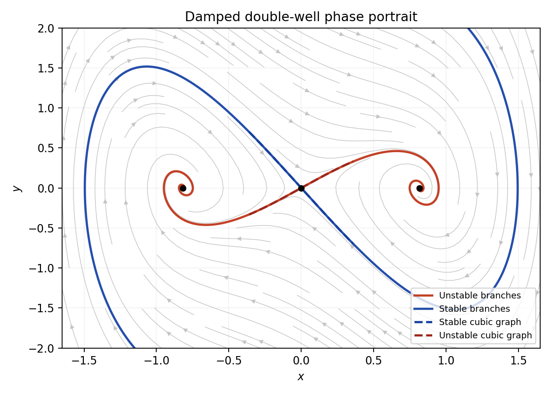
Damped double-well phase portrait: a saddle separates two stable foci, with cubic local invariant manifolds
. Details. At a differentiable fixed point, linear perturbations advance by the Jacobian matrix. A hyperbolic source fixed point of a map has both eigenvalues of modulus greater than one, so nearby perturbations expand under forward iteration of a map. Real signs can cause alternating directions and a complex pair can cause spiral expansion. Eigenvalues on the unit circle are excluded from this linear classification.
A hyperbolic sink fixed point of a map has both Jacobian eigenvalues strictly inside the unit circle. Its iterates locally attract nearby initial states; complex fixed-point multipliers can make the approach spiral. Zero fixed-point multipliers are strongly contracting and can occur for noninvertible maps. A fixed-point multiplier of modulus one requires nonlinear or exact analysis.
A hyperbolic saddle fixed point of a map has one eigenvalue of modulus less than one and one greater than one. The corresponding stable and unstable directions persist locally as invariant sets or manifolds under the usual smoothness and invertibility assumptions. For a noninvertible map a zero stable fixed-point multiplier is possible, and the word saddle fixed point of a map describes forward contraction in one direction and expansion in the other; backward dynamics may not be unique.
A fixed point satisfies . The Jacobian matrix is ; its eigenvalues are the linear fixed-point multipliers used in (i)–(iii).
For the Lozi map, and . At a positive point this gives , and at a negative point . ThereforeThere is no fixed point at , because then and the first component would be one. On an equality boundary the corresponding scalar equation is , so that branch is absent, not a line of fixed points.
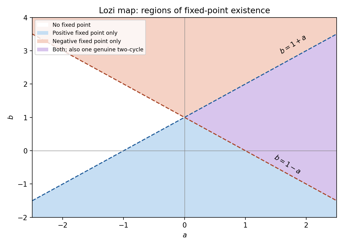
Lozi fixed-point existence regions: positive and negative branches lie in distinct half-planes that can overlap
. Details. For , . If , there is exactly one fixed point unless , when there is none. Its eigenvalues satisfy . It is a sink fixed point of a map for and a source fixed point of a map for . At , the affine map about its fixed point is a quarter turn, and , so it is neutral, not attracting. At no fixed point exists. The positive/negative branch labels follow the sign of .
If , exists for with fixed-point multipliers . It is a sink fixed point of a map for and a forward saddle fixed point of a map for . At the fixed-point multiplier is neutral; on the invariant axis the interval is mapped by , giving two-cycles and the fixed midpoint. The negative point exists only for and has fixed-point multipliers , again a forward saddle fixed point of a map. For there is no fixed point. At , both fixed-point multipliers vanish and two iterates send all initial points to the fixed point.
For a genuine two-cycle let the first coordinates be and put . The two equations are , . If both first coordinates had the same sign , subtracting would give . Since distinct cycle points must have different first coordinates, this contradicts . If one coordinate were zero, the remaining equations would instead force , also excluded. Hence .
Choose . Solving , givesThe required signs hold exactly when . This is the unique two-cycle up to interchanging its two points, under the stipulated nondegeneracy. Borderline parameter lines can carry different degenerate families and were explicitly excluded. These are Lozi fixed points and the alternating-sign two-cycle.
On the invariant biological population interval , the fixed points are and when meaningful. The zero fixed-point multiplier is : extinction attracts for . At , the nonzero branch crosses the origin in the full real-line family, giving a transcritical bifurcation. The nonzero point lies in the biological population interval for and has fixed-point multiplier , so it is stable for and loses stability through at .
Factoring and removing the fixed points gives the two-cycleIts two-step fixed-point multiplier isIt lies between and exactly for . At the upper endpoint it crosses , creating the next period doubling. The two-cycle amplitude tends to zero like at its birth, so the first flip is supercritical. At the equality endpoints linear fixed-point multipliers alone do not establish asymptotic stability.
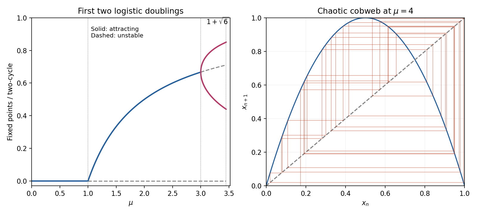


Period-doubling cascade universality concerns the continuation of this period-doubling cascade in smooth unimodal maps with a quadratic maximum. After suitable rescalings their repeated two-step maps approach the same limiting shape; successive parameter spacings have the Feigenbaum ratio approximately and the spatial rescaling has magnitude approximately . These are asymptotic statements involving later doublings, not numbers that can be established from the first two thresholds alone. The accumulation near is outside the first interval considered here. One should not claim chaos throughout the stable two-cycle interval.
Four useful dynamical properties to distinguish are sensitivity to initial conditions, topological transitivity or mixing, dense periodic points, and aperiodic orbits with persistent complex evolution. They concern the invariant set, not an assertion that every orbit must be aperiodic. A positive Lyapunov exponent for typical initial data is an additional quantitative diagnostic.
At , set . The double-angle identity gives the exact solutionFor a direct topological proof use the homeomorphism of . Then , where the full tent map isEvery branch doubles interval length until it crosses a fold; the finite binary cylinders have length and map onto the whole interval after steps. Thus every open interval eventually has an iterate covering the full interval: the map is topologically mixing and sensitive. Repeating a finite left/right branch word gives a periodic itinerary; arbitrarily long prescribed prefixes locate such periodic points in arbitrarily small cylinders, proving density. Nonperiodic binary itineraries yield uncountably many aperiodic orbits. Conjugacy transfers these properties to , proving chaotic behaviour while retaining its dense special periodic orbits.
As a metric check, its invariant measure has density and its typical Lyapunov exponent is . This is a typical-orbit assertion, not a claim about the derivative along every exceptional critical or preperiodic orbit. The explicit trigonometric solution and tent-map conjugacy explain why deterministic iteration of a map can nevertheless amplify uncertainty.
Articles by others on the same topic
There are currently no matching articles.