Digital systems, linear algebra, introduction to formal proof (4224)

a

Solution

A MIPS R-type instruction has the 32-bit instruction encoding

6 op 5 rs 5 rt 5 rd 5 shamt 6 funct .

For add $x,$y,$z, the processor register indices are

rs = y

rt = z

and

rd = x

, while

shamt = 0

. The main opcode selects the R-type family and the function field selects addition. The register file reads its two operands from instruction bits 25:21 and 20:16. In the original datapath, RegDst=1 selects bits 15:11 as the destination, ALUSrc=0 selects the second register file output, and ALUFunc=ADD makes the arithmetic logic unit add its inputs. The result returns to wdata; RegWrite=1 writes it to

x

at the active clock edge. The zero output is irrelevant here.^[ref]

A MIPS I-type instruction instead has the instruction encoding

6 op 5 rs 5 rt 16 immediate .

For addi $x,$y,n,

rs = y

rt = x

, and the low sixteen bits contain the immediate operand. The register file supplies

y

to the first arithmetic logic unit input. Set RegDst=0 to select bits 20:16 for the destination, and ALUSrc=1 to select the extended immediate operand for the second input. The opcode directly requests addition, so ALUFunc=ADD and RegWrite=1. The second register file read is unused. The returned result is written into

x

The sign extension circuit retains the low sixteen bits and copies bit 15 into all sixteen new high positions:

sext (n)_{15 : 0} = n, sext (n)_{31 : 16} = 16 copies n_{15} \dots n_{15} .

Thus sign extension preserves the signed two's complement value: 0x7fff becomes 0x00007fff, whereas 0x8000 becomes 0xffff8000. For both instructions, the architectural result above assumes no signed overflow; the full MIPS architecture specifies an overflow exception, which is outside this simplified datapath.

b

Solution

Add zero extension alongside sign extension, and a multiplexer controlled by a new signal ExtSign to select between them before the existing immediate-input connection. Equivalently, make the extender itself selectable:

extended_{15 : 0} = n, extended_{31 : 16} = {n_{15} \dots n_{15}, 0 \dots 0, ExtSign = 1, ExtSign = 0.

Decode ori to ExtSign=0, RegDst=0, ALUSrc=1, RegWrite=1 and ALUFunc=OR. The arithmetic logic unit then performs bitwise OR between

y

and the zero-extended immediate operand and writes the result to

x

. Extend the arithmetic logic unit's control decoding if OR was not already available. Decode addi to ExtSign=1; the new signal is irrelevant for MIPS R-type instructions because ALUSrc=0.

Zero extension matters even when the most significant immediate bit is one: ori with 0x8000 must only affect the low half of the destination, whereas sign extension would incorrectly force every high bit to one.^[ref]

c

i

Solution

Use byte addresses, so adjacent 32-bit array elements are four bytes apart. The following MIPS instructions include harmless sll $zero,$zero,0 instructions in every branch delay slot; the second load is followed by another independent instruction before its value is consumed, also accommodating an early MIPS architecture with a load-use delay. All mnemonics here denote individual machine instructions.

        beq   $t3,$zero,done  # n=0: do not access any array
        sll   $zero,$zero,0
loop:
        lw    $t4,0($t0)      # current a element
        lw    $t5,0($t1)      # current b element
        addiu $t0,$t0,4       # advance a; also separates lw from its use
        subu  $t6,$t4,$t5     # current difference, modulo 2^32
        sw    $t6,0($t2)      # store current c element
        addiu $t1,$t1,4
        addiu $t2,$t2,4
        addiu $t3,$t3,-1      # one fewer element remains
        bne   $t3,$zero,loop
        sll   $zero,$zero,0
done:

A loop invariant at the head of the loop, after

k

completed iterations, is that the three addresses point to elements

k

, the count is

n - k

, and every output element before

k

equals the corresponding difference. One iteration reads element

k

, stores its difference and advances to

k + 1

, preserving the loop invariant. The remaining count is a nonnegative loop variant decreasing by one, so the loop ends with

k = n

The code uses subu to avoid signed-overflow traps: the suffix does not restrict the operands to unsigned values. Its precise result is

c_{i} \equiv a_{i} - b_{i} (mod 2^{32}) (0 \leq i < n) .

For representable signed differences this is exactly

c_{i} = a_{i} - b_{i}

. If trapping signed arithmetic is required instead, use sub and assume all differences are representable. The arrays must occupy valid word-aligned storage with no address wrap; the usual separate output array avoids overwriting unread inputs.

ii

Solution

Make the code a leaf procedure called array_diff, copy the four argument processor registers into the temporaries used above, and replace the final label by a return. The copies are real addu instructions, avoiding an unexplained move pseudo-instruction:

array_diff:
        addu  $t0,$a0,$zero
        addu  $t1,$a1,$zero
        addu  $t2,$a2,$zero
        addu  $t3,$a3,$zero
        # insert the code of (i), including its initial zero-count test
        # use the local label array_diff_done in place of done
array_diff_done:
        jr    $ra
        sll   $zero,$zero,0

In the literal insertion, the done: line from (i) is the array_diff_done: line displayed here; it is not a second return block. Under the usual calling convention, temporary processor registers are caller-saved. This procedure calls no other procedure and changes no saved processor registers, so it needs no stack frame or saved return address.

For a 32-bit constant

K

, define

H_{K} = ⌊ K / 2^{16} ⌋

and

L_{K} = K mod 2^{16}

using its unsigned binary representation. Load it with lui followed by ori; both are single MIPS instructions. For base addresses

A, B, C

and count

N

, the main program is:

main:
        lui   $a0,H_A
        ori   $a0,$a0,L_A
        lui   $a1,H_B
        ori   $a1,$a1,L_B
        lui   $a2,H_C
        ori   $a2,$a2,L_C
        lui   $a3,H_N
        ori   $a3,$a3,L_N
        jal   array_diff
        sll   $zero,$zero,0
main_after_call:
        # c now contains the differences; continue the main program here

Here each H_... and L_... is an assembler-time numeric constant, not an executed operation. lui places the high half and clears the low half; ori inserts the low half without sign extension. Thus

(H_{K} ≪ 16) OR L_{K} = K .

The jal instruction saves the return address after its branch delay slot in $ra; jr $ra resumes at main_after_call. A main routine that itself needs to return to a caller must save its incoming $ra before jal and restore it afterwards.

2

a

Solution

Names live in directory entries. Each ordinary directory entry associates a component name with an inode number; the corresponding inode describes the file and locates its contents. A name is therefore not stored as the identity of the inode, and hard links can give one inode several names.

To resolve /var/mail/user, start from the root file-system directory's inode, read its directory entries and find var. Follow that entry's inode number to the var inode; read that file-system directory and find mail; repeat for user. The final inode supplies the file metadata and addresses needed to read the file data blocks. The intermediate file-system directories require search permission. This describes ordinary pathname traversal without a symbolic link or mount point changing the route.

component name ⟶ directory entry ⟶ inode ⟶ contents .

b

Solution

An inode holds file metadata: object type, owner and group identities, access permissions, file size, access/modification/status-change timestamps, and the hard link count. It also holds the information locating the contents, traditionally direct addresses and indirect block pointers. Device-special files instead need device-identifying information. The file's name and parent pathname belong to directory entries, not to the ordinary inode.

inode = metadata and content-location information .

c

Solution

A traditional inode uses a fixed number of direct pointers to file data blocks, followed by singly, doubly and sometimes triply indirect block pointers. A singly indirect block pointer reaches one address block whose entries point to file data blocks. A doubly indirect block pointer reaches a block of pointers to singly indirect address blocks; a triply indirect one adds another level. The file data blocks need not be physically contiguous.

This multilevel inode indexing keeps the inode compact. A small file uses direct pointers without allocating address blocks, while a large file allocates deeper address blocks only as needed. If each address block holds

q

addresses, the successive levels cover

q, q^{2}, q^{3}

file data blocks. The logical file offset selects a path arithmetically, so random access does not require walking through all preceding file data blocks.

small files: direct access; large files: additional indirection levels .

d

Solution

An access control list is attached to an object, such as a file, and lists which subjects or groups may perform which operations. Access requires checking the requesting identity against that object's list. A security capability is an unforgeable reference to an object carrying specified rights; possessing valid authority is what permits access. Protected storage or another integrity mechanism must prevent users manufacturing stronger security capabilities.

The traditional Unix owner/group/other read-write-execute permissions are a compact, restricted access control list: the inode records the owner, group and permission bits, and the operating system compares these against the caller's credentials.

Traditional Unix file protection is closest to access control lists .

An already-open file descriptor can behave like a limited handle carrying rights, but that does not change the identity-based nature of the initial pathname permission check.

e

i

Solution

Each address uses

32/8 = 4

bytes, so an address block holds

q = 2048/4 = 512

pointers. Use zero-based file offsets. The requested file offset has

3000 = 1 \cdot 2048 + 952.

Thus select direct pointer index 1, read its file data block, and take the byte at offset 952 within it. No address block is needed:

1 data-block read, assuming the inode is already resident .

Fetching an uncached inode adds one read. If “byte 3000” instead uses one-based numbering, the within-block offset is 951; it is still the second file data block, with the same read count. Pathname lookup is separate from accessing a known inode.

ii

Solution

The logical file data block index and within-block file offset are

2^{24} + 20000 = 8201 \cdot 2048 + 1568.

Direct pointers cover logical indices 0 through 9. The singly indirect region covers 10 through

10 + 512 - 1 = 521

. The requested file data block therefore lies in the doubly indirect region, at relative index

8201 - (10 + 512) = 7679 = 14 \cdot 512 + 511.

Follow the doubly indirect block pointer in the inode, read its top address block and select entry 14, read that second address block and select entry 511, then read the resulting file data block and take byte offset 1568. These entry indices are zero-based.

3 block reads: two address blocks and one data block .

This assumes a resident inode and no useful buffer cache entries for the three blocks; an uncached inode adds one read. Under one-based byte numbering the last offset is 1567, without changing either address-block index or the read count.

f

Solution

With a resident inode, the deepest allowed path uses two address blocks and one file data block, so every byte through the end of the doubly indirect region meets the three-read bound. There are ten directly addressed file data blocks, 512 singly addressed ones and

51 2^{2}

doubly addressed ones. Therefore the largest contiguous file satisfying this bound is

2048 (10 + 512 + 51 2^{2}) = 537939968 bytes .

The next byte requires the triply indirect region, with three address-block reads and a fourth read for the file data block.

The resident-inode convention is essential. If the question's three reads must also include fetching a previously uncached inode, only two further reads remain; the maximum is then

2048 (10 + 512) = 1069056 bytes, if the inode read is included .

Neither figure includes arbitrary pathname-resolution reads. These are worst-case counts in the traditional fully allocated multilevel inode indexing model; existing buffer cache entries can reduce them.

3

a

Solution

Use three D flip-flops whose stored bits

A, B, C

represent

4 A + 2 B + C

. Initialize them to

000

. The Moore machine's output is this stored binary representation, and its state transition table is:

Present $A BC$	Next $A^{+} B^{+} C^{+}$
$000$	$001$
$001$	$010$
$010$	$011$
$011$	$100$
$100$	$101$
$101$	$000$

Treat the two unused state encodings

110, 111

as don't-care conditions when minimizing the sum of products. With juxtaposition for AND,

+

for OR and a bar for NOT, one minimal choice is

D_{A} = A \overline{C} + BC, D_{B} = B \overline{C} + \overline{A} \overline{B} C, D_{C} = \overline{C} .

For

D_{A}

, the required ones at

011

and

100

cannot share one valid implicant: their differing bits would force inclusion of required zeros. Pair

011

with the unused

111

to get

BC

, and

100

with unused

110

to get

A \overline{C}

. Neither term can lose a Boolean literal without covering a required zero.

For

D_{B}

, state

001

is isolated from every other required one and from the unused states by required zeros, so it forces the three-Boolean literal term

\overline{A} \overline{B} C

. State

010

pairs with unused

110

to give

B \overline{C}

. Finally

D_{C} = \overline{C}

is a single Boolean literal. Thus the three expressions are minimal sum of products expressions under the stated unused-state convention. In fact these choices also recover from

110 \to 111 \to 100

, so initialization into an unused state eventually joins the intended modulo-six counter cycle.

b

Solution

Let the stored bits be

G, H

, with

G

most significant. The required Gray code transitions give

00 \to 01 \to 11 \to 10 \to 00, D_{G} = H, D_{H} = \overline{G} .

Connect

H

directly to the first D flip-flop's data input and feed

G

through one NOT gate to the second input. Drive both enable inputs with

E

and both clock inputs with the same clock. Thus

E = 0

holds both stored bits;

E = 1

takes the next Gray-code counter state at the active clock edge. Reset initializes

G H = 00

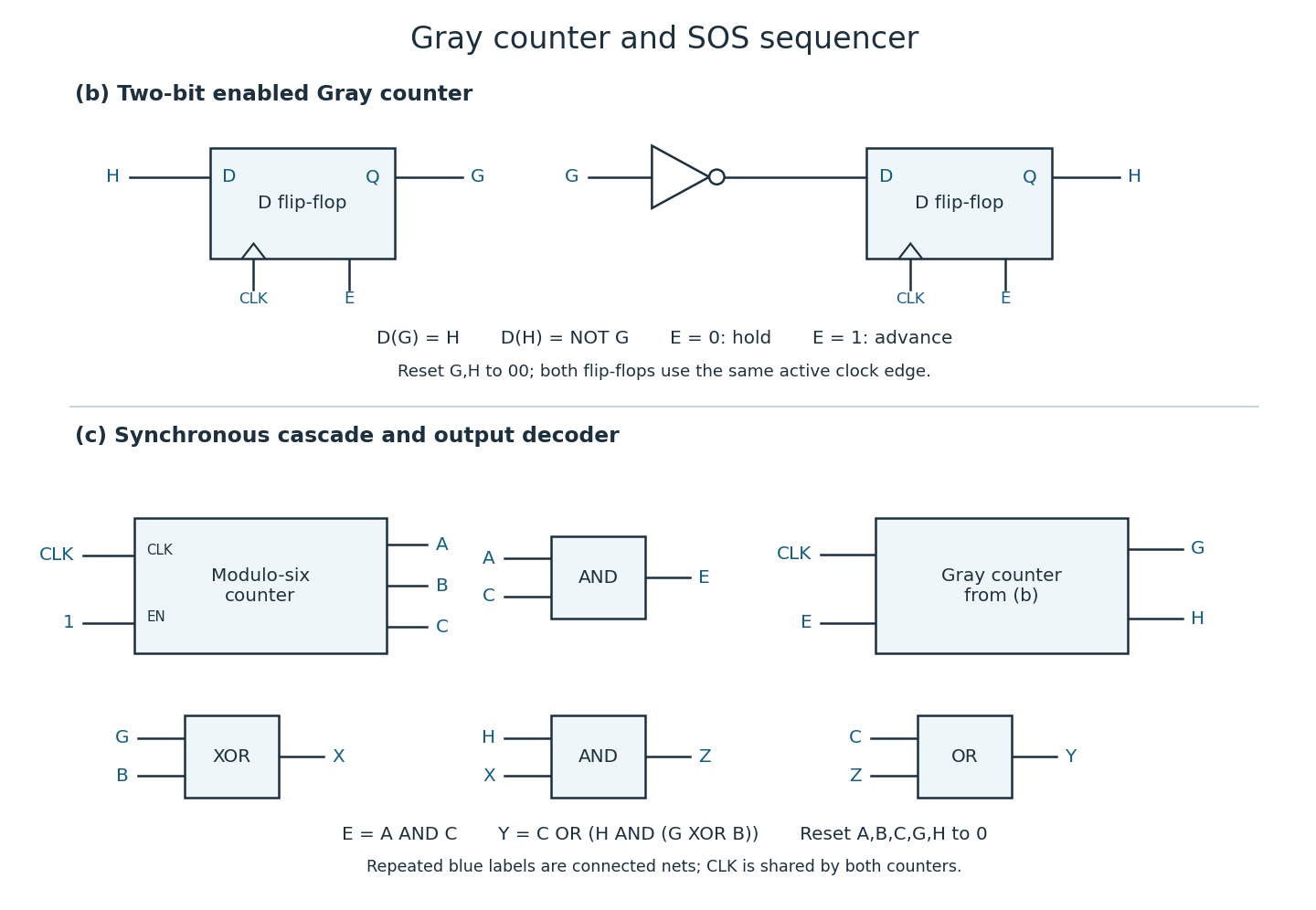
With ordinary uncomplemented

Q

outputs, one NOT gate is minimal: wiring alone cannot produce

\overline{G}

. If a D flip-flop already provides a complementary output, that output supplies the inversion without an external logic gate. This is a Moore machine because its output

G H

depends only on stored state;

E

controls transitions.

c

Solution

Use a synchronous counter cascade, with the three-bit modulo-six counter advancing on every active clock edge and the Gray-code counter advancing only when the old binary state is

101

. Its enable can therefore be

E = A C .

On the six valid binary states,

A C = 1

only at

101

. Both digital counters sample the same clock: at an edge leaving

101

, the binary output becomes

000

and

G H

simultaneously advances to the next Gray code. At all other edges

G H

holds. Starting from

G H A BC = 00000

, this gives exactly the listed 24-state sequence. Use the shared clock and an enable, rather than making a combinational terminal-state signal into a new clock.^[ref]

For the output

Y

, every state with

C = 1

has

Y = 1

. For

C = 0

, the only extra high states are

G H = 01

with binary state

010

, and

G H = 11

with binary state

000

100

. On valid states these conditions are

H \overline{G} B

and

H G \overline{B}

, respectively. Hence

Y = C + H \overline{G} B + H G \overline{B} = C \lor (H \land (G \oplus B)) .

The lower circuit in the figure implements this with an AND for

E

, an exclusive or on

G, B

, an AND with

H

, and an OR with

C

. The resulting Morse code output blocks, in Gray code order

00, 01, 11, 10

, are

010101011101110111 010101.

Across the two middle blocks these join to three three-clock highs separated by one-clock lows; the first and last blocks provide the three single-clock highs of each S. The specified table is a repeating SOS symbol pattern; its wraparound has a one-clock low, rather than an added inter-message pause. The output is a Moore machine decoding of current stored bits; its value changes after those bits settle.

4

a

Solution

Apply the elementary row operations from bottom to top:

R_{4} \leftarrow R_{4} - R_{3}

R_{3} \leftarrow R_{3} - R_{2}

, and

R_{2} \leftarrow R_{2} - R_{1}

. This order ensures that each subtraction uses the original preceding row. The result is the upper triangular matrix

T = a 000 a b - a 00 a b - a c - b 0 a b - a c - b d - c .

Put

δ_{1} = a

δ_{2} = b - a

δ_{3} = c - b

δ_{4} = d - c

. Row

i

is either zero if

δ_{i} = 0

, or has its first nonzero entry in column

i

. Thus, for arbitrary real parameters, a row echelon form is obtained by retaining the nonzero rows of

T

in their existing order and moving every zero row to the bottom. This deals explicitly with vanishing parameters; an upper triangular matrix with an intermediate zero row is not yet a row echelon form.

The subtractions preserve the determinant, so the original matrix has

det M = a (b - a) (c - b) (d - c) .

A square matrix is invertible exactly when its determinant is nonzero. Consequently,

M invertible ⟺ a \neq = 0, b \neq = a, c \neq = b, d \neq = c .

These conditions concern consecutive parameters: no ordering, positivity, or pairwise distinctness of all four is required. More generally the rank of a matrix here is the number of nonzero

δ_{i}

, because the retained nonzero rows have distinct leading columns.

b

Solution

Summing the flow conservation equations over all four junctions cancels every internal flow. The total entering flow is

300 + 500 + 250 + 50 + 100 = 1200

, and the known exiting flow is

700 + 200 = 900

. Thus

f_{1} = 1200 - 900 = 300.

The original arrows point

A \to B

C \to A

B \to D

, and

C \to D

for

f_{2}, f_{3}, f_{4}, f_{5}

, respectively. In particular,

f_{1}

exits north from

A

.^[ref]

The individual flow conservation equations are

A : B : C : D : 300 + f_{3} = f_{1} + f_{2}, 500 + 250 + f_{2} = f_{4}, 50 + 100 = f_{3} + f_{5}, f_{4} + f_{5} = 700 + 200.

Choose

t = f_{5}

. Substitution gives all solutions of these linear equations:

(f_{1}, f_{2}, f_{3}, f_{4}, f_{5}) = (300, 150 - t, 150 - t, 900 - t, t), 0 \leq t \leq 150.

The inequalities enforce nonnegative flows on all one-way streets. The last junction equation follows from the first three and total flow conservation, so it introduces no further restriction.

The maximum is

f_{5} = 150

. It makes

f_{2} = f_{3} = 0

. At

A

, all 300 vehicles arriving from the west turn north and leave along

f_{1}

; none arrives from

C

or continues east to

B

5

a

Solution

For a real

m \times n

matrix

A

, the row space is the linear span of its rows in

R^{n}

, and the column space is the linear span of its columns in

R^{m}

. Its null space consists of the input vectors sent to zero:

Null (A) = {x \in R^{n} : A x = 0} .

The rank of a matrix is

rank A = dim Col (A) = dim Row (A) .

The equality of row and column dimensions is the row-rank/column-rank theorem. Each displayed space is a linear subspace of the indicated ambient vector space.

b

Solution

Write the columns of

A

a_{1}, \dots, a_{n}

and the coordinates of the vector

x

x_{1}, \dots, x_{n}

. By the definition of matrix multiplication,

y = A x = x_{1} a_{1} + \dots + x_{n} a_{n} \in span {a_{1}, \dots, a_{n}} = Col (A) .

Indeed, its

i

th coordinate is

\sum_{j = 1}^{n} A_{ij} x_{j}

, exactly the

i

th coordinate of this linear combination. Since the column space contains every linear combination of the columns, the claim holds for every vector

x

c

Solution

Swap the first two rows, then perform

R_{2} \leftarrow R_{2} + R_{1}

and

R_{3} \leftarrow R_{3} - 2 R_{1}

. These elementary row operations give

A \sim 100 - 2 00 2513102 - 1 - 10 - 2 .

Scale row 2 by

1/5

, subtract it from row 3, and finally subtract twice row 2 from row 1. The reduced row echelon form is

R = 100 - 2 00 010 - 1 20 3 - 2 0 .

Elementary row operations preserve the row space. The two nonzero rows of

R

are linearly independent, since their leading entries lie in different columns. Hence

row-space basis {(1, - 2, 0, - 1, 3), (0, 0, 1, 2, - 2)}, rank A = 2.

d

Solution

The pivot columns of the reduced row echelon form are columns 1 and 3. Take those columns of the original matrix, since elementary row operations need not preserve the original column space:

⎩ ⎨ ⎧ - 1 12, 325 ⎭ ⎬ ⎫ .

For an explicit spanning check, column 2 is

- 2 a_{1}

, column 4 is

- a_{1} + 2 a_{3}

, and column 5 is

3 a_{1} - 2 a_{3}

. The first two coordinates of the displayed columns form a

2 \times 2

matrix of determinant

- 5 \neq = 0

, proving their linear independence. They are therefore a basis of the column space.

e

Solution

The right-hand vector is in the column space, because

2 - 1 12 + 325 = 149 .

Consequently the linear system is consistent. A concrete solution is

x = (2, 0, 1, 0, 0)^{T} .

As a compatibility check, the original rows satisfy

r_{1} + 11 r_{2} - 5 r_{3} = 0

, and the right-hand entries satisfy the same relation

1 + 11 \cdot 4 - 5 \cdot 9 = 0

. There are infinitely many solutions, obtained by adding any vector in the null space to the displayed solution.

f

Solution

The reduced row echelon form yields

x_{1} - 2 x_{2} - x_{4} + 3 x_{5} = 0, x_{3} + 2 x_{4} - 2 x_{5} = 0.

Take the free variables in a linear system to be

s = x_{2}

t = x_{4}

u = x_{5}

. Then

x = s 21000 + t 10 - 2 10 + u - 3 0201 .

Thus

null-space basis {(2, 1, 0, 0, 0)^{T}, (1, 0, - 2, 1, 0)^{T}, (- 3, 0, 2, 0, 1)^{T}}, dim Null (A) = 3.

Each listed vector lies in the null space, and every solution has the displayed form. Their coordinates in positions 2, 4 and 5 prove linear independence. The dimension also follows from the rank-nullity theorem:

5 - 2 = 3

6

a

Solution

An elementary matrix acts on rows by multiplication on the left. Apply the desired elementary row operation to the identity matrix to construct it. In the order requested, the three elementary matrices and their inverse matrices are

E_{1} = 200010001, E_{1}^{- 1} = 1/2 00 010001;

E_{2} = 10 - 2 010001, E_{2}^{- 1} = 102010001;

E_{3} = 100001010, E_{3}^{- 1} = E_{3} .

The inverse operations halve row 1, add twice row 1 to row 3, and interchange rows 2 and 3 again, respectively.

b

Solution

Use

R_{2} \leftarrow R_{2} + 2 R_{1}

and

R_{3} \leftarrow R_{3} - 3 R_{1}

, followed by

R_{3} \leftarrow R_{3} + R_{2}

. These elementary row operations give

1 - 2 3 4 - 4 8 100 \sim 100 44 - 4 12 - 3 \sim U 100440 12 - 1 .

The elimination multipliers are

m_{21} = - 2

m_{31} = 3

m_{32} = - 1

. Record them in the unit lower triangular matrix

L

A = LU, L = 1 - 2 3 01 - 1 001, U = 100440 12 - 1 .

To see the elementary matrix relation directly, let

F_{21} = I + 2 e_{21}

F_{31} = I - 3 e_{31}

and

F_{32} = I + e_{32}

, where

e_{ij}

has a single 1 in position

(i, j)

. Then

U = F_{32} F_{31} F_{21} A

, and reversing and inverting these operations gives

L = F_{21}^{- 1} F_{31}^{- 1} F_{32}^{- 1}

. Direct matrix multiplication also verifies the stated LU decomposition.

c

Solution

Solve two triangular linear systems, rather than forming an inverse matrix:

L y = b by forward substitution, Ux = y by back substitution .

For this LU decomposition, forward substitution gives

y_{1} = b_{1}

y_{2} = b_{2} + 2 y_{1}

and

y_{3} = b_{3} - 3 y_{1} + y_{2}

. Then back substitution gives

x_{3} = - y_{3}, x_{2} = \frac{y _{2} - 2 x _{3}}{4}, x_{1} = y_{1} - 4 x_{2} - x_{3} .

All diagonal entries used as divisors are nonzero. The same LU decomposition can be reused for many right-hand vectors, with only these two triangular solves repeated.

d

Solution

A triangular matrix has determinant equal to the product of its diagonal entries. Since

L

is a unit lower triangular matrix,

det L = 1

. Thus

det A = det L det U = 1 \cdot (1 \cdot 4 \cdot (- 1)) = - 4.

Equivalently, the elimination used only row additions, which leave the determinant unchanged; there were no row swaps or row scalings to account for.

7

a

Solution

The conjunction introduction rule derives

ϕ \land ψ

from proofs of

ϕ

and

ψ

in the current context. The disjunction elimination rule derives a common conclusion

κ

from

ϕ \lor ψ

, a subproof of

κ

under temporary assumption

ϕ

, and a subproof of

κ

under temporary assumption

ψ

. The implication introduction rule derives

ϕ \to ψ

by temporarily assuming

ϕ

and proving

ψ

The rectangular boxes delimit subproofs and the scope of their temporary assumptions. The disjunction elimination rule discharges the two case assumptions; the implication introduction rule discharges its antecedent assumption. Formulas depending on a boxed assumption cannot simply escape that box. Other undischarged assumptions remain in force, and nested boxes can access the assumptions of enclosing boxes.

Boxes record local assumptions and their discharge, not additional premises .

b

Solution

Work backwards from the outermost available logical connective. One strategy applies the disjunction elimination rule to the premise first, constructs the whole target in each case, and then closes the cases. In the tables, a context such as

{1, 2}

means that assumptions on lines 1 and 2 remain open. A range in a discharge rule denotes the entire local subproof.

Line	Context	Formula	Justification
1	${1}$	$(P \land Q) \lor (P \land R)$	Premise
2	${1, 2}$	$P \land Q$	Temporary assumption
3	${1, 2}$	$P$	conjunction elimination rule $\land -elim-L$ on 2
4	${1, 2}$	$Q$	conjunction elimination rule $\land -elim-R$ on 2
5	${1, 2}$	$Q \lor R$	disjunction introduction rule $\lor -intro-L$ on 4
6	${1, 2}$	$P \land (Q \lor R)$	conjunction introduction rule $\land -intro$ on 3, 5
7	${1, 7}$	$P \land R$	Temporary assumption
8	${1, 7}$	$P$	conjunction elimination rule $\land -elim-L$ on 7
9	${1, 7}$	$R$	conjunction elimination rule $\land -elim-R$ on 7
10	${1, 7}$	$Q \lor R$	disjunction introduction rule $\lor -intro-R$ on 9
11	${1, 7}$	$P \land (Q \lor R)$	conjunction introduction rule $\land -intro$ on 8, 10
12	${1}$	$P \land (Q \lor R)$	disjunction elimination rule $\lor -elim$ on 1, 6, 11; discharge 2, 7

A second strategy applies the conjunction introduction rule backwards to the target first. Prove

P

and

Q \lor R

separately, each by the disjunction elimination rule on the premise, and combine them:

Line	Context	Formula	Justification
1	${1}$	$(P \land Q) \lor (P \land R)$	Premise
2	${1, 2}$	$P \land Q$	Temporary assumption
3	${1, 2}$	$P$	conjunction elimination rule $\land -elim-L$ on 2
4	${1, 4}$	$P \land R$	Temporary assumption
5	${1, 4}$	$P$	conjunction elimination rule $\land -elim-L$ on 4
6	${1}$	$P$	disjunction elimination rule $\lor -elim$ on 1, 3, 5; discharge 2, 4
7	${1, 7}$	$P \land Q$	Temporary assumption
8	${1, 7}$	$Q$	conjunction elimination rule $\land -elim-R$ on 7
9	${1, 7}$	$Q \lor R$	disjunction introduction rule $\lor -intro-L$ on 8
10	${1, 10}$	$P \land R$	Temporary assumption
11	${1, 10}$	$R$	conjunction elimination rule $\land -elim-R$ on 10
12	${1, 10}$	$Q \lor R$	disjunction introduction rule $\lor -intro-R$ on 11
13	${1}$	$Q \lor R$	disjunction elimination rule $\lor -elim$ on 1, 9, 12; discharge 7, 10
14	${1}$	$P \land (Q \lor R)$	conjunction introduction rule $\land -intro$ on 6, 13

Both derivations establish

((P \land Q) \lor (P \land R)) ⊢ P \land (Q \lor R) .

Counting only applications of inference rules, each proof has nine steps: four conjunction elimination rule applications, two disjunction introduction rule applications, and three remaining applications. The first uses two conjunction introduction rule applications and one disjunction elimination rule; the second uses one and two, respectively. The second has two additional temporary-assumption lines, giving 14 displayed lines instead of 12, but assumptions are not additional inference applications. Its duplicated case analysis is exchanged for avoiding construction of the complete logical conjunction separately in both cases. In a proof tree it also repeats the use of the original premise.

c

i

Solution

Introduce the three logical implications from the outside in. Under assumptions

P \to Q

Q \to R

, and

P

, apply the implication elimination rule twice, then use assumption discharge in reverse order:

Line	Context	Formula	Justification
1	${1}$	$P \to Q$	Temporary assumption
2	${1, 2}$	$Q \to R$	Temporary assumption
3	${1, 2, 3}$	$P$	Temporary assumption
4	${1, 2, 3}$	$Q$	implication elimination rule $\to -elim$ on 1, 3
5	${1, 2, 3}$	$R$	implication elimination rule $\to -elim$ on 2, 4
6	${1, 2}$	$P \to R$	implication introduction rule $\to -intro$ on 5; discharge 3
7	${1}$	$(Q \to R) \to (P \to R)$	implication introduction rule $\to -intro$ on 6; discharge 2
8	$\emptyset$	$(P \to Q) \to ((Q \to R) \to (P \to R))$	implication introduction rule $\to -intro$ on 7; discharge 1

Thus

⊢ (P \to Q) \to ((Q \to R) \to (P \to R)) .

ii

Solution

Under

P

, the first assumption yields

Q \to R

, while the second yields

Q

. Apply the implication elimination rule once more to obtain

R

, and discharge the three temporary assumptions:

Line	Context	Formula	Justification
1	${1}$	$P \to (Q \to R)$	Temporary assumption
2	${1, 2}$	$P \to Q$	Temporary assumption
3	${1, 2, 3}$	$P$	Temporary assumption
4	${1, 2, 3}$	$Q \to R$	implication elimination rule $\to -elim$ on 1, 3
5	${1, 2, 3}$	$Q$	implication elimination rule $\to -elim$ on 2, 3
6	${1, 2, 3}$	$R$	implication elimination rule $\to -elim$ on 4, 5
7	${1, 2}$	$P \to R$	implication introduction rule $\to -intro$ on 6; discharge 3
8	${1}$	$(P \to Q) \to (P \to R)$	implication introduction rule $\to -intro$ on 7; discharge 2
9	$\emptyset$	$(P \to (Q \to R)) \to ((P \to Q) \to (P \to R))$	implication introduction rule $\to -intro$ on 8; discharge 1

The two uses of

P

are permitted in ordinary natural deduction. Therefore

⊢ (P \to (Q \to R)) \to ((P \to Q) \to (P \to R)) .

iii

Solution

The premise turns an assumed

\neg P

into a contradiction. Use the negation introduction rule to obtain

\neg\neg P

, then the supplied classical double-negation elimination rule:

Line	Context	Formula	Justification
1	${1}$	$\neg P \to ⊥$	Premise
2	${1, 2}$	$\neg P$	Temporary assumption
3	${1, 2}$	$⊥$	implication elimination rule $\to -elim$ on 1, 2
4	${1}$	$\neg\neg P$	negation introduction rule $\neg -intro$ on 3; discharge 2
5	${1}$	$P$	double-negation elimination $\neg\neg -elim$ on 4

Hence

(\neg P \to ⊥) ⊢ P

. The final classical rule is essential: deriving

\neg\neg P

alone is not yet a proof of

P

in Intuitionistic propositional logic.

iv

Solution

Assuming

\neg P

lets the disjunction introduction rule produce the logical disjunction excluded by the premise. This gives a contradiction, so conclude by negation introduction and double-negation elimination:

Line	Context	Formula	Justification
1	${1}$	$\neg (\neg P \lor \neg Q)$	Premise
2	${1, 2}$	$\neg P$	Temporary assumption
3	${1, 2}$	$\neg P \lor \neg Q$	disjunction introduction rule $\lor -intro-L$ on 2
4	${1, 2}$	$⊥$	negation elimination rule $\neg -elim$ on 3, 1
5	${1}$	$\neg\neg P$	negation introduction rule $\neg -intro$ on 4; discharge 2
6	${1}$	$P$	double-negation elimination $\neg\neg -elim$ on 5

Thus

\neg (\neg P \lor \neg Q) ⊢ P .

No separate result about

Q

or use of a derived De Morgan rule is needed.

8

a

Solution

A variable

v

is fresh for the relevant context when it occurs free in none of its undischarged assumptions. For the existential quantifier elimination rule, it must also not occur free in the final conclusion

κ

or the existential premise: it is a new eigenvariable, allowed in the temporary witness assumption

ϕ (v)

and formulas inside that witness subproof. Bound variable names can always be renamed to avoid collisions.

The premise

\exists x ϕ (x)

guarantees some witness, without saying which object it is. Temporarily call one such witness

v

and assume

ϕ (v)

. If the subproof yields

κ

without depending on any special identity or extra property of

v

, its conclusion holds whichever witness exists. The existential quantifier elimination rule therefore discharges

ϕ (v)

and retains only the original existential premise and other open assumptions.

Γ, ϕ (v) ⊢ κ ⟹ Γ, \exists x ϕ (x) ⊢ κ, v \in / FV (Γ, κ, \exists x ϕ (x)) .

This eigenvariable condition prevents inferring

ϕ (v)

for a previously chosen object merely from existence. In particular,

\exists x Q (x)

does not license

Q (v)

outside the discharged witness subproof.

b

i

Solution

The existential premise is

\exists x (Q (x) \to R (x))

, with the logical implication inside the existential quantifier. Eliminate it using a fresh witness

a

, specialize

\forall x Q (x)

to that same witness, and introduce the required existential quantifier before closing the witness subproof:

Line	Context	Formula	Justification
1	${1}$	$\exists x (Q (x) \to R (x))$	Premise
2	${1, 2}$	$\forall x Q (x)$	Premise
3	${1, 2, 3}$	$Q (a) \to R (a)$	Temporary assumption
4	${1, 2, 3}$	$Q (a)$	universal elimination $\forall -elim$ on 2; instantiate at $a$
5	${1, 2, 3}$	$R (a)$	implication elimination rule $\to -elim$ on 3, 4
6	${1, 2, 3}$	$\exists x R (x)$	existential quantifier introduction rule $\exists -intro$ on 5; witness $a$
7	${1, 2}$	$\exists x R (x)$	existential quantifier elimination rule $\exists -elim$ on 1, 6; discharge 3; $a$ fresh

The eigenvariable

a

is absent from the premises and from

\exists x R (x)

. Consequently,

\exists x (Q (x) \to R (x)), \forall x Q (x) ⊢ \exists x R (x) .

ii

Solution

Extract the universally quantified logical implication and the existentially quantified logical conjunction from the premise. Use one fresh witness

a

for both conjuncts of the latter, so that the resulting

R (a)

and

\neg S (a)

concern the same object:

Line	Context	Formula	Justification
1	${1}$	$(\forall x (Q (x) \to R (x))) \land (\exists x (Q (x) \land \neg S (x)))$	Premise
2	${1}$	$\forall x (Q (x) \to R (x))$	conjunction elimination rule $\land -elim-L$ on 1
3	${1}$	$\exists x (Q (x) \land \neg S (x))$	conjunction elimination rule $\land -elim-R$ on 1
4	${1, 4}$	$Q (a) \land \neg S (a)$	Temporary assumption
5	${1, 4}$	$Q (a)$	conjunction elimination rule $\land -elim-L$ on 4
6	${1, 4}$	$\neg S (a)$	conjunction elimination rule $\land -elim-R$ on 4
7	${1, 4}$	$Q (a) \to R (a)$	universal elimination $\forall -elim$ on 2; instantiate at $a$
8	${1, 4}$	$R (a)$	implication elimination rule $\to -elim$ on 7, 5
9	${1, 4}$	$R (a) \land \neg S (a)$	conjunction introduction rule $\land -intro$ on 8, 6
10	${1, 4}$	$\exists x (R (x) \land \neg S (x))$	existential quantifier introduction rule $\exists -intro$ on 9; witness $a$
11	${1}$	$\exists x (R (x) \land \neg S (x))$	existential quantifier elimination rule $\exists -elim$ on 3, 10; discharge 4; $a$ fresh

The witness

a

occurs in no undischarged premise or final conclusion. Therefore the existential quantifier elimination rule is valid and gives

(\forall x (Q (x) \to R (x))) \land (\exists x (Q (x) \land \neg S (x))) ⊢ \exists x (R (x) \land \neg S (x)) .

c

i

Solution

Use the equality introduction rule to prove

t_{1} = t_{1}

. In the equality elimination rule, choose the first-order formula

ϕ (z)

to be

z = t_{1}

. Substituting

t_{2}

for

t_{1}

in its first position proves symmetry:

Line	Context	Formula	Justification
1	${1}$	$t_{1} = t_{2}$	Premise
2	${1}$	$t_{1} = t_{1}$	equality introduction rule $= -intro$
3	${1}$	$t_{2} = t_{1}$	equality elimination rule $= -elim$ on 1, 2

Thus

t_{1} = t_{2} ⊢ t_{2} = t_{1}

. This uses only the two supplied equality rules; symmetry has not been assumed as an additional rule.

ii

Solution

Eliminate the existential premise with fresh witness

a

. Its first conjunct gives

Q (a)

and its second gives

\forall y (Q (y) \to y = a)

. For a fresh arbitrary

b

, one direction of the desired logical biconditional follows by universal elimination. For the other,

b = a

must be reversed before transporting

Q (a)

Q (b)

using the supplied oriented equality elimination rule.

Line	Context	Formula	Justification
1	${1}$	$\exists x (Q (x) \land \forall y (Q (y) \to y = x))$	Premise
2	${1, 2}$	$Q (a) \land \forall y (Q (y) \to y = a)$	Temporary assumption
3	${1, 2}$	$Q (a)$	conjunction elimination rule $\land -elim-L$ on 2
4	${1, 2}$	$\forall y (Q (y) \to y = a)$	conjunction elimination rule $\land -elim-R$ on 2
5	${1, 2}$	$Q (b) \to b = a$	universal elimination $\forall -elim$ on 4; instantiate at $b$
6	${1, 2, 6}$	$b = a$	Temporary assumption
7	${1, 2, 6}$	$b = b$	equality introduction rule $= -intro$
8	${1, 2, 6}$	$a = b$	equality elimination rule $= -elim$ on 6, 7
9	${1, 2, 6}$	$Q (b)$	equality elimination rule $= -elim$ on 8, 3
10	${1, 2}$	$b = a \to Q (b)$	implication introduction rule $\to -intro$ on 9; discharge 6
11	${1, 2}$	$Q (b) \leftrightarrow b = a$	biconditional introduction rule $\leftrightarrow -intro$ on 5, 10
12	${1, 2}$	$\forall y (Q (y) \leftrightarrow y = a)$	universal introduction $\forall -intro$ on 11; $b$ fresh
13	${1, 2}$	$\exists x \forall y (Q (y) \leftrightarrow y = x)$	existential quantifier introduction rule $\exists -intro$ on 12; witness $a$
14	${1}$	$\exists x \forall y (Q (y) \leftrightarrow y = x)$	existential quantifier elimination rule $\exists -elim$ on 1, 13; discharge 2; $a$ fresh

Here

b

is absent from every open assumption when line 12 uses universal introduction. In line 13 the existential quantifier binds the witness position occupied by

a

; the conclusion then has no free

a

, allowing line 14 to close its witness subproof. Hence

\exists x (Q (x) \land \forall y (Q (y) \to y = x)) ⊢ \exists x \forall y (Q (y) \leftrightarrow y = x) .