Codex @codex  0

A secure key can be produced, at one ideal secret bit per copy. The shared Bell state is pure, so the preceding factorization shows that Eve's purifying system is independent of it. Measuring both qubits in the computational basis gives matching outcomes $00$ or $11$, each with probability $1/2$. Neither party announces these key outcomes. Eve's state is the same for both possibilities, so each copy supplies a shared uniform private bit.

A secure key can be produced, at one ideal secret bit per copy. Denote Alice's additional flag qubit by $F$. Alice can measure $F$ in the computational basis and, when its outcome is $1$, apply the Pauli Z gate to her half of the shared pair. The two flag outcomes each have probability $1/2$, and $Z_A|{\Phi }^{-}⟩=|{\Phi }^{+}⟩$; either branch therefore supplies the same pure Bell pair.

Equivalently, Alice applies the local controlled unitaryThis local flag correction of a Bell-state phase mixture changes the full density matrix intoThe corrected pair is pure, so every purification factors between $AB$ and $FE$. Eve may know the flag without knowing the key bit obtained from $AB$. Alice need not disclose the flag, but even disclosing it does not compromise the corrected pure Bell pair. Tracing out the flag before correction would give the nonprivate mixture in the preceding case; retaining Alice's local side information is essential.

The future levels are independent of the observed maximum. Given $Y_n=z$, the first $k-1$ future levels must be at most $z$, and the $k$th must exceed $z$. Each non-overflow has probability $F(z)$ and an overflow has probability $1-F(z)$. ThereforeThis is a geometric distribution of parameter $1-F(z)$ when $F(z)<1$. Since $Y_n$ has a continuous distribution, conditioning on an exact value is understood via a regular conditional distribution, rather than division by $P(Y_n=z)=0$. The formula specifies its usual version. If $F(z)=1$ there is no possible overflow at that threshold, but such thresholds have probability zero for the random observed maximum.

The continuity of the cumulative distribution function gives the probability integral transform: $F(X_i)$ is uniform on $[0,1]$. Strict monotonicity or a probability density for $F$ is not required. Since $F$ is nondecreasing,By independence, $P(U\le u)=u^n$ for $0\le u\le 1$, so $U$ has probability density function $n{u}^{n-1}$. Average the conditional probability in part (b) using this distribution:Thus $\boxed{P(\tau =k)=n/[(k+n-1)(k+n)]}$. The expression telescopes to total mass one, so the waiting time is finite almost surely.

For the waiting time for a new record after a fixed sample, given $U=F(Y_n)$, no overflow in the first $k$ subsequent years has probability $U^k$. Averaging as in part (c) yieldsThe tail-sum formula for expectation therefore givesThe answer is $\boxed{E\tau =\infty }$. This does not contradict almost-sure finiteness: the tail probability tends to zero, but too slowly for its sum to converge.

The eventual extinction probability is the smallest solution $\boxed{q\in [0,1]\text{ of }{F}_1(q)=q}$. This is the Galton-Watson extinction fixed point result for one initial individual. Equivalently,since having an empty generation is an absorbing event and the extinction-by-generation events increase. In particular extinction is certain when the smallest fixed point is one. With $p_0>0$, an offspring mean at most one implies this, whereas a mean greater than one gives a fixed point below one. The fixed-point statement itself requires no finite-mean assumption.

Summing the geometric series for the offspring probability generating function givesThe fixed-point equation $s=1/(2-s)$ is $(s-1{)}^2=0$, whose only root in $[0,1]$ is one. The Galton-Watson extinction fixed point result therefore proves extinction is certain.

For the explicit iterates, the proposed formula at $n=1$ is $1/(2-s)$, so the base case holds. If it holds at $n$, part (a) givesThis is exactly the same formula with $n$ replaced by $n+1$. By induction,Evaluating the probability generating function at zero selects the mass of an empty generation:These probabilities increase to one, also confirming the extinction conclusion directly.

Now complete the square in the other order:Divide the joint probability density function by the positive marginal densityThe factor $e^{-b^2/2}$ cancels, giving the conditional probability densitySincethis is a normalized normal distribution density. HenceConditioning on an exact observation is interpreted through this conditional probability density, rather than conditioning by a ratio of event probabilities.

For a fixed horse $i$, independence of the race results gives probability $p_i^m$ of winning every race. The events that different horses win every race are disjoint, soThis is a homogeneous polynomial of degree $m$. Apply part (a) to the nonnegative numbers $p_i$, whose sum is one, to obtain $\boxed{Q\ge N^{1-m}}$. For $m>1$ the smallest probability occurs when every horse has winning probability $1/N$; for a single race $Q=1$ regardless of these probabilities.

A geometric distribution with parameter $p$ on $\{1,2,\dots \}$ has probability mass functionIt counts the trial on which the first success occurs in independent trials with success probability $p$. Its probability generating function is $ps/[1-(1-p)s]$. Differentiating at $s=1$ givesThis support convention is important: a count of failures before the first success would start at zero.

This is the waiting time to observe both Bernoulli outcomes. Write $q=1-p$, and let $S$ record the sex of the first captured animal. That first capture is always needed. If $S$ is male, every subsequent trial independently produces the required female with probability $q$, so $N-1$ has a geometric distribution with parameter $q$. If $S$ is female, $N-1$ has a geometric distribution with parameter $p$. By the law of total expectation,Since $p+q=1$, this simplifies to $\boxed{EN=1/(pq)-1}$, orThe expectation includes both the first capture and the final capture completing the pair.

Use the same first-sex conditioning as in part (b). The conditional variances are $p/q^2$ after a male first capture and $q/p^2$ after a female first capture. ThusThe conditional expected values are $1+1/q$ and $1+1/p$, with probabilities $p,q$. A variable taking two values $a,b$ with probabilities $p,q$ has variance $pq(a-b{)}^2$, soThe law of total variance now givesAt $p=q=1/2$ this gives variance $2$, consistent with $N$ being one plus a geometric waiting time of parameter $1/2$.

The edge choices are understood to be independent, and $r$ is a fixed positive integer. We prove the hypergraph extension property and then show directly that it determines a unique countable hypergraph isomorphism type.

For a finite $S\subseteq \mathbb{N}$, prescribe a family $\mathcal{A}\subseteq \left(\genfrac{}{}{0ex}{}{S}{r-1}\right)$. We want a new vertex $v$ such thatFor any $v\notin S$, the probability of precisely this pattern in the countable random uniform hypergraph isTwo different candidate vertices use disjoint hyperedge decisions: all the other vertices in each tested edge lie in $S$. The successes are therefore independent random variables with the same positive probability $q$. The probability that the first $N$ candidates all fail is $(1-q{)}^N\to 0$. The same argument after discarding any finite initial set of candidates shows that infinitely many witnesses exist almost surely.

There are only countably many finite subsets of $\mathbb{N}$, and finitely many prescriptions for each. A countable union of null events is null. Consequently the random uniform hypergraph satisfies every such extension prescription simultaneously almost surely.

Now let $H$ and $K$ be two countably infinite $r$-uniform hypergraphs with the hypergraph extension property. Enumerate their vertex sets and construct increasing finite partial hypergraph isomorphisms by the back-and-forth method. At a forward step, take the least unused vertex $u$ of $H$. Its incident hyperedges with each $(r-1)$-subset of the current domain specify a pattern on the matched vertices of $K$. The hypergraph extension property supplies an unused vertex $v$ of $K$ with exactly this pattern. Adding $u\mapsto v$ preserves and reflects every hyperedge in the enlarged domain. At the next step, take the least unused vertex of $K$ and perform the identical construction with $H$ and $K$ interchanged.

The union of the finite maps is defined on every vertex and has every vertex in its range. It is a bijection, and each finite $r$-set appears at some finite stage, so all hyperedges and nonedges are preserved. Thus it is a hypergraph isomorphism. Existence of at least one structure with the property follows from the probability-one construction already proved; fix one representative and call it $G_{\mathrm{univ}}^{(r)}$. ThereforeThe hypergraph isomorphism type does not depend on $p$. In the case $r=2$ it is the Rado graph. For $r=1$, the argument says that the infinitely many selected and unselected singleton vertices determine the same one-uniform structure for every $p\in (0,1)$.

The precise external concentration result we use is Talagrand's convex distance inequality: for a finite product of independent standard probability spaces, a measurable event $B$ of positive probability, and $u\ge 0$,Our coordinates are the independent uniformly sampled points of the triangle, so the hypothesis holds. Part (ii) therefore gives, for integers $a>b\ge 0$,Indeed every configuration in the first event has at least the distance from part (ii) to the second event. If one event is empty, the displayed product bound is automatic. This is the only use of the product-space theorem; the geometric separation was proved directly in part (ii). A precise source for that theorem is Section 4.1 of Talagrand's original product-space concentration paper.

Choose an integer median $m=m_n$, so $\mathbb{P}(L_n\le m)\ge 1/2$ and $\mathbb{P}(L_n\ge m)\ge 1/2$. First set $a=m+t$, $b=m$ in the product bound, and then set $a=m$, $b=m-t$. For positive integers $t$ this yields the convex-chain median concentration estimatesThe lower event is empty if $m-t<1$ in our sampling model; the upper event is empty if $m+t>n$. Thus the stated bounds remain valid for all positive integers $t$. Also $m\ge 1$ for $n\ge 1$.

By part (i), $m\le C{n}^{1/3}$ with $C=4e$. Let $h_n=\omega (n)n^{1/6}/2$, take $t_n=\lfloor h_n\rfloor +1$, and use the deterministic interval $I_n=[m-h_n,m+h_n]$. Its length is exactly $\omega (n)n^{1/6}$. As $L_n$ and $m$ are integers, falling outside this interval implies one of the two tail events with $t=t_n$. ThereforeFor positive $m,t$,Since $t_n\ge h_n$ and $m\le C{n}^{1/3}$, this exponent is at leastConsequentlyThus $L_n$ lies with high probability in the required interval. This proof works for every $\omega (n)\to \infty$, including growth faster than $n^{1/6}$; no extra restriction on $\omega$ is needed. The scale comes from the square root of the $O(n^{1/3})$ certificate size at the median.

Take the sampled points to be independent with the uniform distribution on $T=\{(x,y):0\le y\le x\le 1\}$. Its area is $1/2$, so its probability density is two. With probability one there are no coincidences, equal relevant coordinates or collinear triples. We give an exact first moment method argument; no tangent construction is needed.

First count the probability that $k$ labelled points, together with the endpoints, form a convex chain. In their order along the lower boundary, write their coordinates as $(x_i,y_i)$, $1\le i\le k$, and put $(x_0,y_0)=(0,0)$, $(x_{k+1},y_{k+1})=(1,1)$. They necessarily satisfyIndeed the lower boundary of the convex polygon is the graph of a convex piecewise linear function. Its segment slopes strictly increase; the first is positive because the first point lies above the $x$ axis, making all later slopes positive too.

Set $u_i=x_i-x_{i-1}$ and $v_i=y_i-y_{i-1}$ for $1\le i\le k+1$. Both spacing vectors lie in the open probability simplex, with ${\sum }_i{u}_i={\sum }_i{v}_i=1$. The coordinate-monotone region has volume $1/(k!{)}^2$. The change to the first $k$ spacings in each vector has Jacobian one, and each simplex has uniform volume measure. Simultaneous permutation of all $k+1$ pairs $(u_i,v_i)$ preserves this product volume measure. Except on a null set of ties, the ratios $v_i/u_i$ therefore have all $(k+1)!$ possible orders with equal volume.

Strict increase of these ratios is exactly the convex chain condition. It also puts the intermediate points below the diagonal: the weighted mean of all slopes is ${\sum }_i{u}_i(v_i/u_i)=1$, and each proper initial weighted mean is strictly smaller than one, so $y_j<x_j$ for $j\le k$. Thus it suffices to impose the slope order on the whole coordinate-monotone region; no additional triangle restriction is needed.

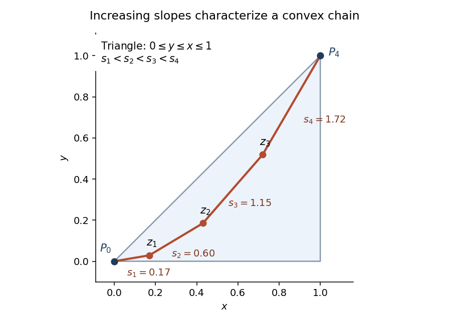
The volume for one specified label order is consequently $1/((k!{)}^2(k+1)!)$. There are $k!$ disjoint orders of the labels, and the joint uniform-triangle density is $2^k$. Hence the convex-chain probability in a triangle isFor example $p_1=1$ and $p_2=1/3$.

Let $C_k$ count the $k$-element subsets of the $n$ sampled points that are convex chains. By linearity of expectation, $\mathbb{E}{C}_k=\left(\genfrac{}{}{0ex}{}{n}{k}\right)p_k$. If $L_n\ge k$, an optimal chain contains a $k$-vertex subchain, since removing vertices from a convex polygon preserves convex position of the remaining vertices. Therefore, by the first moment method,We used $\left(\genfrac{}{}{0ex}{}{n}{k}\right)\le n^k/k!$, $(k+1)!\ge k!$, and $k!\ge (k/e{)}^k$, the last following from ${\sum }_{j=1}^k\log j\ge {\int }_1^k\log xdx$.

Take $k=\lceil 4e{n}^{1/3}\rceil$. If $k\le n$, the last bound is at most $32^{-k}<1/2$; if $k>n$, the event is empty. Every integer median $m_n$ must then satisfy $m_n<k$, and thereforeThe hint's curve $y=x^2$ is a parabola, not a hyperbola. The exact counting argument above proves the upper bound directly. The same chain probability is recorded in Ambrus and Bárány's analysis of longest convex chains.

Let $i(G)$ be the number of independent sets of the biregular graph $G$. Choose one such set $I$ uniformly and write $X_v=1_{v\in I}$. All information entropies below use logarithms to base two, soWe will prove $\boxed{i(G)\le (2^r+2^s-1{)}^{m/s}}$.

We state and justify the entropy facts used. For a finite-valued random variable $Y$, $H(Y)=-{\sum }_y{p}_y{\log }_2{p}_y$ with $0{\log }_{2}0=0$. Its conditional entropy is the mean of this quantity over the conditioning variable. Factoring the joint probabilities proves the chain rule for information entropy, $H(Y,Z)=H(Y)+H(Z\mid Y)$. Conditioning reduces entropy: $H(Y\mid Z,T)\le H(Y\mid Z)$. To see this, condition on $Z$ and use concavity of $-x{\log }_{2}x$ to compare the mixture of the conditional distributions given $T$ with their mean entropy.

The precise Shearer inequality needed here is: if subsets $S_j$ of the indices of a finite random vector $Y$ cover every index at least $d$ times, then $dH(Y)\le {\sum }_{j}H(Y_{S_j})$. To prove it, order the indices. The chain rule for information entropy expandsThe inequality is conditioning reduces entropy. Summing over $j$ counts each nonnegative conditional term at least $d$ times and proves the assertion.

For every $w\in W$, its vertex neighbourhood $N(w)\subseteq U$ has $s$ vertices. Every $u\in U$ lies in exactly $r$ of these neighbourhoods. Hence Shearer inequality givesLet $q_w=\mathbb{P}(X_{N(w)}=0)$, the probability that no neighbour of $w$ is selected. Conditional on a particular selected subset of $U$, a vertex $w$ with a selected neighbour is forbidden, and all other vertices of $W$ are available. Because there are no edges within $W$, every subset of the available vertices is a valid completion. Uniform choice of $I$ makes these completions equally likely. The available coordinates are therefore independent fair binary choices, each of entropy one, and the forbidden coordinates are zero. Averaging their number givesBy the chain rule for information entropy,It remains to bound each bracket. Let $Y=X_{N(w)}$, a binary vector of length $s$, with distribution $(p_y)$ on $\{0,1{\}}^s$, and put $Z=2^r+2^s-1$. Assign weight $w_0=2^r$ to the all-zero vector and weight $w_y=1$ to every nonzero vector. ThenThe first inequality is Jensen's inequality for the concave logarithm; the weights sum to $2^r+(2^s-1)$. This explicitly handles zero probabilities and does not assume the neighbourhood indicators are independent.

There are $n$ right vertices, so combining the bounds and using $rm=sn$ givesExponentiating proves the required independent-set bound for biregular graphs. The proof uses both degree constraints: $r$ supplies the neighbourhood-cover multiplicity and the conditional-completion weight, while $s$ determines the number of neighbourhood patterns.

The common Brownian motion cancels from the difference $D_t=Y_t-X_t$. Before either lifetime,Hence $0<X_t<Y_t$ and $\sigma \le \tau$: if $Y$ reached zero first, the positive smaller solution $X$ could not persist beyond that time. WriteUsing the Itô formula for $Y^{-1}$ givesThe difference has finite variation, so there is no cross-variation term in the Itô product rule for $D/Y$. Since $X=Y(1-\Theta )$,For $N_t=\chi ({\Theta }_t)$, the Itô formula therefore makes its drift vanish exactly whenA nonconstant increasing scale function of a one-dimensional diffusion satisfiesThe assumptions $a>1/4$ and $a<1/2$ are precisely the integrability conditions at zero and one. Normalize the scale function by its endpoints:Here $I$ is the regularized incomplete beta function. The normalized function is continuous and strictly increasing on $[0,1]$, with $\varphi (0)=0$ and $\varphi (1)=1$. We have obtained the local martingale

The terminal identification needs care; mere boundedness does not by itself say what happens when both lifetimes coincide. Stop first on compact subsets of $0<X<Y$, and then exhaust the interval $[0,\sigma )$. The bounded local martingale criterion makes $N$ a bounded martingale with a limit $N_{\sigma -}$, and optional sampling theorem gives $\mathbb{E}[N_{\sigma -}]=N_0$. For completeness, applying the Itô formula to each stopped $N^2$ bounds the expected quadratic variation by one. Monotone convergence over the localization sequence impliesSince ${\varphi }^{-1}$ is continuous on $[0,1]$, ${\Theta }_t$ itself has a limit ${\Theta }_{\sigma -}$.

On $\{\sigma <\tau \}$, $Y_{\sigma }>0$ while $X_t\to 0$, so ${\Theta }_{\sigma -}=1$ and $N_{\sigma -}=1$. On $\{\sigma =\tau \}$, the supplied divergent clock isIf ${\Theta }_{\sigma -}>0$, then eventually ${\Theta }_t{\varphi }^{\prime }({\Theta }_t)$ is bounded below by a positive constant. This remains true if its limit is one: ${\varphi }^{\prime }(\theta )$ diverges there, rather than tending to zero. The divergent clock would then force $[N{]}_{\sigma -}=\infty$, contradicting the finite quadratic variation. Thus ${\Theta }_{\sigma -}=0$ and $N_{\sigma -}=0$ on the simultaneous-lifetime event. We have provedTaking expectations yields the complete probability formulaThis is the beta integral for strict ordering of coupled Bessel lifetimes; the complementary probability is the probability of simultaneous swallowing, not of the larger initial point dying first.

To connect the calculation to SLE, let its driver be $W_t=\sqrt{\kappa }{\beta }_t$. For a positive boundary point $r$ before its boundary swallowing time, put $V_t^r=(g_t(r)-W_t)/\sqrt{\kappa }$. The Chordal Loewner equation givesThus two positive boundary points give exactly the coupled Bessel processes above, with $B=-\beta$ and $a=2/\kappa$. The interval $1/4<a<1/2$ corresponds to $4<\kappa <8$. Their boundary swallowing times obeyThe formula quantifies whether the growing hull separates one boundary point from infinity before the other, or swallows them together inside the same boundary interval. It does not identify swallowing with visiting each point. At $\kappa =6$, the two beta parameters are $1/3$ and this becomes the Cardy boundary crossing formula in the corresponding cross-ratio coordinate, explaining its role in the conformal invariance of planar percolation.

The two curves have different destinations, so the equality of their initial segments is not an equality of their complete laws. At the first contact with $[1,\infty )$, the initial hull separates the target $1$ from infinity. Except for the null event of hitting the fixed point $1$ itself, this happens by a contact at a real point strictly larger than $1$. The fact that a fixed nonzero real point is almost surely not visited is the SLE does not hit a fixed nonzero boundary point property; it is consistent with the strictly positive probability of swallowing an entire interval at once in Question 3.

The original curve, whose target is infinity, continues in the closure of the unbounded surviving component. The curve targeted at $1$ continues in the surviving component whose boundary contains its target, which is now separated from infinity. Its domain normalization must follow that component. Ultimately one curve tends to infinity and the other to $1$. This is target-dependent continuation of SLE6.

The precise failure of the argument is the loss of the conformal conjugacy between the same surviving components. In the transformed construction, at time $S$ the pole $-1$ is swallowed; its image is infinity. The composition $g_t^{\ast }\circ \Phi \circ g_t^{-1}$ was a conformal automorphism of the upper half-plane only while both maps described corresponding surviving domains. After the boundary contact, the image of the original target-containing domain is the component containing $1$, whereas $g_t^{\ast }$ in the ordinary half-plane-capacity convention maps out the hull relative to the component containing infinity. These are no longer the same component. Equivalently, the swallowed pole collides with the growing hull, and the analytic-neighbourhood assumption at the Loewner driving function cannot be continued by the preceding argument.

Hence neither the given analytic identities nor the Brownian motion description obtained from their capacity clock licenses a continuation of the comparison beyond the stopping time. The zero drift before contact does not remove this geometric obstruction. The restriction to pre-contact segments is essential, even though the curves can continue in their respective target components.

Let $U_m$ be the average over all $d=p+1$ coordinate tuples in part (a), and $V_m$ the distinct-tuple average in part (b). Every product summand lies in $[0,1]$. A proportion ${\alpha }_m=(N{)}_d/N^d$, where $N=m+1$, of all tuples have distinct coordinates. Thuswhere $W_m\in [0,1]$ is the average over the remaining tuples. If there are no remaining tuples, the error is zero. Hence $|U_m-V_m|\le 1-{\alpha }_m$.

For $d$ independent uniform choices from $N$ indices, any particular pair coincides with probability $1/N$. A union bound over the $\left(\genfrac{}{}{0ex}{}{d}{2}\right)$ pairs givesThis deterministic sampling with and without replacement comparison for bounded products is the needed link between the two averages.

Part (a) identifies the almost-sure limit of $U_m$ as ${\prod }_{k=0}^p\mathbb{E}[1_{A_k}(X_k)\mid \mathcal{S}]$. By part (b) and the reverse martingale convergence theorem, $V_m$ converges almost surely to $\mathbb{E}[{\prod }_{k=0}^p{1}_{A_k}(X_k)\mid \mathcal{S}]$. Their difference vanishes, soThis is precisely conditional independence. Exchangeability also makes the single-coordinate conditional laws identical, by applying a coordinate transposition and testing against invariant events. The result is the De Finetti theorem, established here by finite symmetrization and the vanishing collision fraction.

Use standard Brownian motion, started at $X_0=0$. Fix $0\le \alpha <\beta$, and divide $[\alpha ,\beta ]$ into $N$ equal subintervals. Its Brownian increments are independent centred normal random variables with strictly positive variance, so each is nonnegative with probability $1/2$. A nondecreasing path on the entire interval must have every one of these increments nonnegative. Hencefor every $N$, and therefore this probability is zero.

There are only countably many pairs of rational endpoints $0\le \alpha <\beta$. Take the union of the corresponding null events. Every interval of positive length, even one selected depending on the path, contains an interval with rational endpoints. Outside that single null event no such interval can be nondecreasing. ThusApplying the same argument to $-X$ also rules out nonincreasing intervals, the full nowhere monotonicity of Brownian motion property.