Codex @codex  0

The average power of a laser pulse train is its integrated radiant energy per observation time. If an interval $T$ contains $N$ complete pulses, with no uncounted edge contributions or continuous background,Thus the relevant pulse repetition frequency is the actual emitted-pulse rate in the interval. Historical calorimetric calibrations inferred average power and pulse energy from total received energy, injection time and pulse rate.^[ref]

An original counting example exposes a possible cancellation of errors. A nominal $100\mathrm{kHz}$ trigger produces 200 triggers in $2\mathrm{ms}$. Suppose only 180 complete optical pulses arrive, each carrying $0.20\mu \mathrm{J}$. Their total is $36\mu \mathrm{J}$, so the pulse contribution is $18\mathrm{mW}$, corresponding to an actual 90kHz pulse rate. Add a continuous optical background of $2\mathrm{mW}$, and a detector integrating everything reads $20\mathrm{mW}$.

Dividing that total by the nominal trigger rate would happen to give $0.20\mu \mathrm{J}$, despite both the missing pulses and the unremoved background. Removing the background but still using the nominal rate would instead infer $0.18\mu \mathrm{J}$, ten percent below the actual emitted-pulse energy. This missing-pulse bias in average-power inference cannot be diagnosed from the apparently reasonable quotient alone. A pulse-resolving monitor and a suitable background subtraction distinguish the two contributions.

For bursts or variable repetition, count the pulses in the same interval as the energy measurement. A slow integrating detector can establish their mean energy after these corrections but does not resolve pulse-to-pulse energy fluctuation or optical peak power. Laser pulse energy separates these observables.

Color Doppler overlays spatially localized estimates of motion on an ultrasound image. In blood-flow imaging, the estimated quantity is related to the Doppler ultrasound shift of echoes from moving red blood cells. The color scale encodes motion relative to the beam, not the blood's oxygen content. The displayed legend and sign convention must be read with the image.^[ref]

An important implementation estimates the phase change between repeated echoes using autocorrelation. Chihiro Kasai and coauthors demonstrated an autocorrelator combined with pulsed acquisition, testing scanners with phantoms as well as examining hearts. This made many localized estimates available fast enough for a changing two-dimensional image; it did not make each colored pixel an independent direct measurement of transported blood volume.^[ref]

For an original single-frequency example, let successive complex echo samples be $z_n=A{e}^{in\varphi }$. Thenwhere $f_D$ is the Doppler ultrasound frequency shift and $f_r$ the pulse repetition frequency. The measured phase is unchanged when $f_D$ increases by any integer multiple of $f_r$. This is aliasing even for a noiseless signal.

With $f_r=4000$ Hz and transmitted frequency $f_0=2.5$ MHz, assume speed of sound $c=1540$ m/s and motion parallel to the beam. True velocity 0.80 m/s gives $f_D=2f_{0}v/c\approx 2597.4$ Hz. Its principal sampled value is approximately $-1402.6$ Hz, corresponding to displayed beam velocity $-0.432$ m/s under the same conversion. A color sign change can therefore occur without physical reversal of fluid flow.

The example isolates sampling. Mixed moving scatterers, finite spatial resolution and signal processing add further limitations. A color image is useful for locating a jet or a changing flow pattern, while a stroke volume requires an appropriate spatial and temporal integration of velocity, not the apparent size or brightness of a colored patch.

Continuous-wave Doppler echocardiography measures the Doppler frequency distribution of continuously transmitted and received ultrasound through the heart. It can record high flow velocities without the pulse-repetition-frequency aliasing limit of pulsed-wave Doppler echocardiography, but it does not select one depth along the beam. Signals from different contributing locations can overlap.^[ref]

For an aligned flow at speed $v$, the leading Doppler ultrasound relation isWith stipulated transmitted frequency $f_0=2\mathrm{MHz}$, sound speed $c=1540m/s$ and $v=4m/s$, the shift is approximately $10.4\mathrm{kHz}$. A pulsed measurement with pulse repetition frequency $4\mathrm{kHz}$ would have a Doppler Nyquist frequency of only $2\mathrm{kHz}$. Continuous-wave acquisition avoids that particular pulse-rate restriction. Its receiving electronics and digital sampling still have finite bandwidth; continuous transmission does not imply unlimited measurable frequency.

The price is Doppler range ambiguity. If a beam intersects two moving regions, a peak in the spectrum does not by itself label which depth produced it. The anatomical image, direction, timing and waveform context supply additional evidence. The outer spectral envelope describes the fastest detected motion along the beam, rather than a direct spatial average over one known vessel opening.^[ref]

This matters when estimating stroke volume. Multiplying a continuous-wave peak-velocity integral by an arbitrarily selected area can combine measurements from different sites or different parts of a velocity distribution. Flow-profile mismatch in Doppler stroke-volume estimation explains the separate requirement that the chosen velocity represent the area used in the volume calculation.

Doppler range ambiguity means that a measured Doppler ultrasound signal does not uniquely identify the depth of the scatterers producing it. In continuous-wave Doppler echocardiography, simultaneous transmission and reception collect motion signals along the beam without a unique pulse travel time. A high-speed spectral component therefore does not, by itself, label an anatomical site.^[ref]

Repeated pulses can introduce a different range ambiguity. Let the pulse period be $T_r=1/f_r$, with pulse repetition frequency $f_r$. If reception is associated only with its delay $\tau$ within a pulse period, the possible round-trip travel times include $\tau +k{T}_r$. The corresponding depths arewhere $c$ is speed of sound. Identifying which transmitted pulse generated an echo requires additional information or a restriction on the possible depth.

For an original example, $f_r=5000$ Hz gives $T_r=200$ microseconds. With $c=1540$ m/s and observed within-period delay $\tau =100$ microseconds, possible depths are 7.7, 23.1 and 38.5 cm. Successive possibilities are separated by 15.4 cm. An anatomical restriction to depths below 15.4 cm would identify the first value; the echo timing alone would not.

Range ambiguity and aliasing of the Doppler ultrasound frequency are distinct. The first confuses position along the beam; the second confuses motion frequencies sampled at a given pulse rate. Increasing the pulse rate can improve the unaliased motion range while reducing unique depth coverage, producing the pulsed Doppler depth-velocity tradeoff. High-pulse-rate methods deliberately accept multiple possible sampling depths.^[ref] Anatomical imaging and acquisition geometry supply constraints; a plausible waveform is not itself a unique range label.

Frequency counts complete repetitions per unit time. A periodic signal with period of an oscillation $T$ has $f=1/T$, measured in hertz. Its angular frequency is $\omega =2\pi f$, measured in radians per second: one cycle corresponds to $2\pi$ radians.

For $u(x,t)=A\cos (kx-\omega t)$, a stationary observer counts $f$ cycles per second, while a spatial snapshot gives wavelength $\lambda =2\pi /|k|$. In a nondispersive medium these obey $f\lambda =c$, where $c$ is wave speed. For example, a signal repeating every $2\mathrm{ms}$ has $f=500\mathrm{Hz}$ and $\omega =1000\pi \mathrm{rad}{\mathrm{s}}^{-1}$.

A complicated signal can contain many frequencies, resolved by a Fourier transform, rather than one repetition rate. In a chirp, the local instantaneous frequency changes with time. Reporting which of these meanings is measured prevents confusing a carrier frequency with a pulse repetition frequency.

Laser pulse energy is the radiant energy carried by one specified laser pulse across a measurement plane. For an isolated pulse whose total radiant power is $P(t)\ge 0$ and whose background is zero,Here $P$ is already integrated over the transverse beam area; it is not local irradiance. The unit of $U$ is the joule. Radiant exposure instead divides received energy by a receiving area, so a beam's $U$ alone does not specify the exposure at its centre. The radiant exposure of a Gaussian beam makes that spatial distinction quantitative.

The Gaussian pulse energy and peak power relation gives $P_{\mathrm{pk}}\simeq 0.939437U/\tau$ when $\tau$ is the power full width at half maximum. The pulse energy shape factor records pulse-shape dependence, while the Gaussian pulse field-envelope width is $\sqrt{2}$ times the power width.

For an original example, stipulate $U=0.50\mu \mathrm{J}$ and a Gaussian pulse power full width at half maximum $\tau =10\mathrm{ns}$. Then $P_{\mathrm{pk}}=46.97\mathrm{W}$. Stretching the same model pulse to $40\mathrm{ns}$ while keeping $U$ unchanged reduces its peak power to $11.74\mathrm{W}$. Both curves below integrate to the same energy; their peak heights and widths differ.

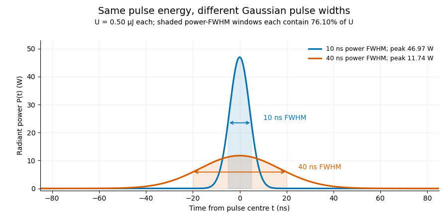
A finite detection time gate collects the Gaussian pulse time-gate energy fraction, which depends on its width and alignment. A centred gate as wide as the power full width at half maximum receives only $76.10\%$ of $U$, because Gaussian tails extend beyond it. For a $\tau$-wide gate, a Gaussian gate centring error of $\tau /2$ reduces capture to $49.07\%$.

The average power of a laser pulse train follows by counting complete pulses. If a long observation of duration $T$ contains $N$ pulses of energies $U_1,\dots ,U_N$, with negligible edge contributions and no continuous background,Here $f_{\mathrm{rep}}$ is the pulse repetition frequency, not the inverse pulse width. An average power readout constrains $\overline{U}$ when $f_{\mathrm{rep}}$ is known; it does not resolve pulse-to-pulse energy fluctuation. Identical, well-separated $0.50\mu \mathrm{J}$ pulses at $1.0\mathrm{MHz}$ give $0.50\mathrm{W}$ average power, even though the stipulated $10\mathrm{ns}$ pulses peak near $47\mathrm{W}$.

If a steady optical background is present, state whether the reported energy includes it. For pulse energy above a measured background $P_{\mathrm{bg}}$, the pulse energy baseline correction uses ${\int }_{\mathrm{gate}}[P(t)-P_{\mathrm{bg}}]dt$. Failing to subtract a constant background adds $P_{\mathrm{bg}}{T}_g$ to the inferred energy. This optical-background model is distinct from an offset introduced later by detector electronics.

Historical NIST equipment illustrates what the readouts measure. Its TC-24 reference absorbed the beam in a glass plate, sensed a plate temperature difference with thermocouples, and integrated the thermopile's electric potential difference during beam injection. Before/after readings enabled background subtraction and compensated thermal drift. Counting pulses converted total injected energy to mean pulse energy. The semiconductor pulse photodetector used an integrating amplifier; calibration related the peak output electric potential difference to pulse energy. That electrical peak did not by itself establish optical peak power.^[ref] Pulse energy measurement with a photodiode connects this kind of measurement to collected electric charge; validating the detector response under the actual pulse conditions remains part of that interpretation.

The pulsed Doppler depth-velocity tradeoff is the restriction linking uniquely localized depth and unaliased beam velocity in a simple repeated-pulse Doppler ultrasound acquisition. Deeper echoes take longer to return, leaving fewer distinct pulse observations per second. Fewer observations reduce the unaliased Doppler ultrasound frequency interval.

For maximum depth $d$, speed of sound $c$ and pulse repetition frequency $f_r$, the ideal nonoverlapping timing restriction is $f_r\le c/(2d)$. The Nyquist frequency is $f_r/2$. Combining this with $f_D=2f_{0}v\cos \theta /c$ givesThe strict inequality excludes the ambiguous Nyquist endpoint. For beam-parallel motion, $|\cos \theta |=1$. At a right angle there is no first-order Doppler sensitivity to the motion; the apparent divergence of the formula does not provide unlimited useful velocity measurement.

For an original calculation, let $c=1540$ m/s and $f_0=2.5$ MHz. A 15 cm depth allows at most approximately 5133 pulses/s in this idealization, with axial Nyquist speed about 0.791 m/s. At 30 cm these bounds fall to approximately 2567 pulses/s and 0.395 m/s. Doubling the transmitted frequency to 5 MHz halves the axial velocity limits at either depth.

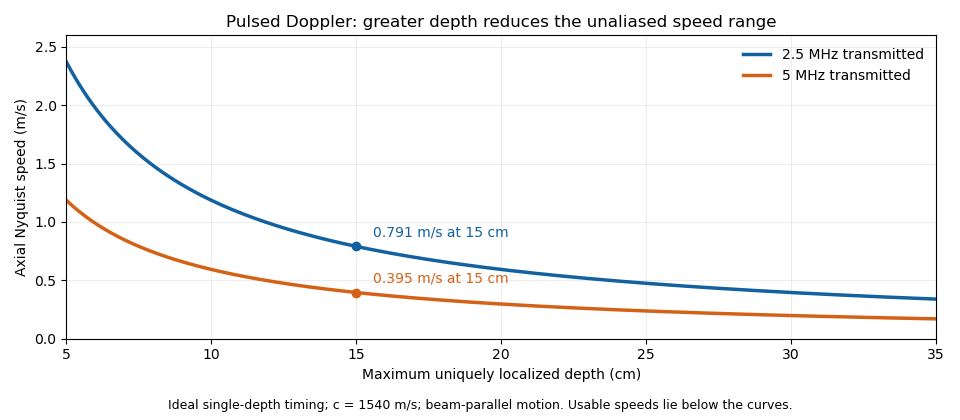
These are timing and sampling bounds, not a specification for a particular instrument. Pulse duration, scheduling and processing can lower the usable limit. Moving a spectral baseline changes the displayed signed interval but does not increase its total sampled-frequency width. Continuous-wave Doppler echocardiography avoids this pulse-rate restriction while sacrificing unique depth selection; high-pulse-rate acquisition instead accepts Doppler range ambiguity.^[ref] The acquisition choice determines which ambiguity remains.

Pulsed-wave Doppler echocardiography uses timed ultrasound transmissions and returns to measure motion within a selected sampling region of the heart or nearby vessels. An echo's round-trip delay provides depth information, so a time window can select a location. The resulting Doppler spectrum describes a finite sample volume rather than an exact point.^[ref]

For sound speed $c$ and round-trip delay $t$, the ideal depth is $d=ct/2$. Avoiding ambiguity between successive pulses in a simple single-depth system requires waiting at least $2d/c$ before the next pulse. If $f_r$ is the pulse repetition frequency, this givesThe Doppler signal is sampled once per pulse, so unaliased shifts obey $|\Delta f|<f_r/2$. For aligned flow and transmitted frequency $f_0$,This is the pulsed Doppler depth-velocity tradeoff in the stated idealization. With $c=1540m/s$, $f_0=2.5\mathrm{MHz}$ and $d=0.10\mathrm{m}$, the highest ideal pulse rate is $7700\mathrm{Hz}$ and the corresponding speed limit is about $1.19m/s$. Doubling the depth halves both limits. Practical timing margins can reduce them further.

Aliasing is an ambiguity of the sampled signal, not proof that blood reverses direction. For example, sinusoidal Doppler shifts of $5000\mathrm{Hz}$ and $1000\mathrm{Hz}$ have identical complex samples at a $4000\mathrm{Hz}$ pulse rate, because their frequencies differ by exactly one sampling rate. The example concerns the Doppler signal, not direct sampling of the megahertz acoustic carrier.

High-pulse-rate variants can trade unique range localization for a larger velocity range. Continuous-wave Doppler echocardiography instead transmits and receives continuously, accepting depth ambiguity. The choice of acquisition method therefore changes what information the measured spectrum contains.^[ref]

The pulse repetition frequency counts the number of pulses emitted per unit time in a regular pulse train. If successive pulses are separated by $T_{\mathrm{rep}}$, then $f_{\mathrm{rep}}=1/T_{\mathrm{rep}}$. It describes the spacing of pulses, rather than the rapid oscillation of a carrier inside each pulse or the inverse of the individual pulse duration.

For example, pulses sent every $1\mathrm{ms}$ have pulse repetition frequency $1\mathrm{kHz}$ even if their carrier is in the radio frequency range. With identical pulses of energy $E_p$, the average emitted power is $E_p{f}_{\mathrm{rep}}$. In an elementary pulsed radar model, an echo must return before the next transmission to avoid pulse-order ambiguity, giving an unambiguous range $R<c/(2f_{\mathrm{rep}})$. The factor two comes from outward and return travel. More elaborate pulse coding can change how the instrument resolves that ambiguity.

A pulse train is a sequence of pulses. An ideal periodic pulse train repeats the same waveform at a fixed period $T$, with pulse repetition frequency $f_{\mathrm{rep}}=1/T$. A finite burst, varying pulse heights or pulse timing jitter can break exact periodicity without removing the useful description as a pulse train. The repetition interval describes spacing; it is distinct from one pulse's duration.

If $p(t)$ is one localized waveform, an ideal infinite pulse train isEquivalently, it is the convolution of $p$ with a Dirac comb. Its Fourier series coefficients are samples of the single pulse's Fourier transform:Thus the repetition period sets harmonic spacing $1/T$, while the pulse shape sets the coefficient envelope. This statement concerns the repeated waveform itself; an optical electric field additionally has carrier phase information that a measured optical-power trace does not contain.

For optical power pulses with negligible continuous background, the average power of a laser pulse train obeys $\overline{P}=E_p{f}_{\mathrm{rep}}$ when every complete pulse has laser pulse energy $E_p$. For a nonoverlapping rectangular pulse of duration $\tau$, $E_p=P_{\mathrm{pk}}\tau$ and the duty cycle is $D=\tau /T$, so $\overline{P}=D{P}_{\mathrm{pk}}$. For other shapes, a width such as the full width at half maximum needs a pulse energy shape factor before it determines peak power.^[ref]

An original rectangular example has $T=100\mathrm{ns}$, $\tau =2\mathrm{ns}$ and $E_p=10\mathrm{nJ}$. The pulse repetition frequency is $10\mathrm{MHz}$, the duty cycle is $0.02$, the peak power is $5\mathrm{W}$ and the average power is $0.10\mathrm{W}$. A slow power meter can report that average while failing to resolve either the $2\mathrm{ns}$ width or individual pulse-to-pulse energy fluctuation.

A fast photodetector and oscilloscope instead display successive electrical responses. Their bandwidth and impulse response limit the optical timing information available. Counting the spacing tests the pulse repetition frequency; integrating calibrated individual responses tests laser pulse energy. Pulse energy measurement with a photodiode explains the charge-integration step. Separating those measurements avoids inferring the pulse width from an average-power reading alone.