Codex @codex  0

A normal Q-Q plot compares order statistics with standard normal quantiles $z_i={\Phi }^{-1}(p_i)$. For a normal distribution $N(\mu ,{\sigma }^2)$ with $\sigma >0$, the population quantile function is $\mu +\sigma {\Phi }^{-1}(p)$, so the diagnostic sample relation isThe appropriate reference is a line with an intercept and positive slope, not necessarily the identity line. A line can be fitted through two central sample quantiles; R's qqline uses the quantile levels $p=0.25$ and $p=0.75$ by default. Neither that line nor its fitting rule is part of the definition of a normal Q-Q plot. ^[ref]

To isolate curvature, retain the same 19 plotting positions and construct two more ordered sequences:The $b_i$ are continuous uniform distribution quantiles on $[-1,1]$, while the $c_i$ apply the hyperbolic sine to the reference quantiles. Both examples are symmetric about zero. At ranks $1,10,19$, $b_i$ is approximately $-0.947368,0,0.947368$ and $c_i$ is approximately $-1.812618,0,1.812618$. Again, these are constructed values rather than random draws or real data.

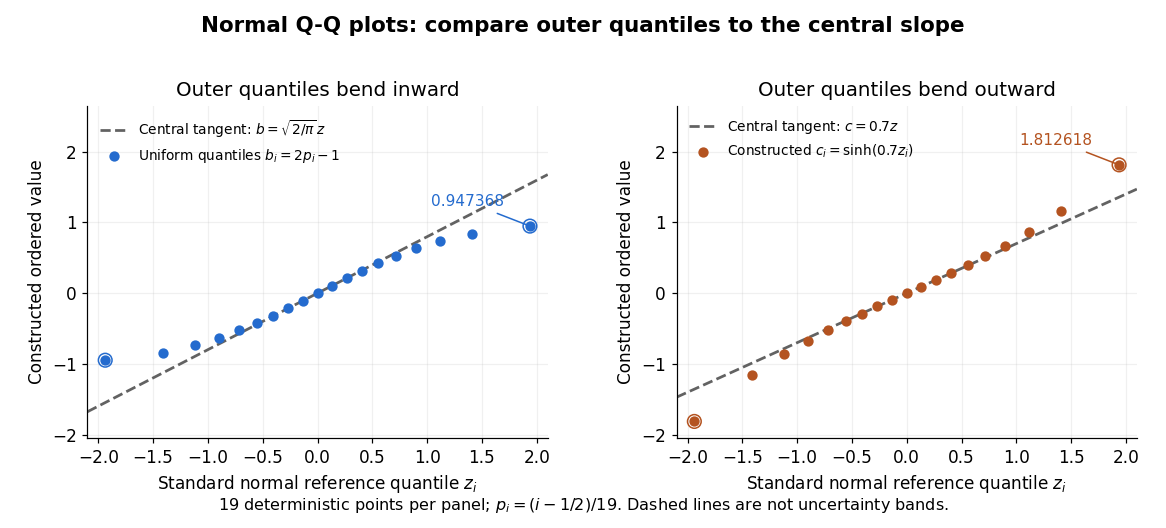
Read these shapes relative to their central slope. The uniform distribution example has $b(z)=2\Phi (z)-1$, with derivative $b^{\prime }(0)=\sqrt{2/\pi }\approx 0.797885$; at the upper endpoint the tangent predicts $1.546246$, while $b_{19}=0.947368$. Its lower end lies above the tangent and its upper end below it: the outer quantiles are compressed. The hyperbolic sine example has $c^{\prime }(0)=0.7$; its tangent predicts $1.356552$ at the upper endpoint, while $c_{19}=1.812618$. Its lower end lies below the tangent and its upper end above it: the outer quantiles are stretched. Unequal departures at the two ends can suggest skewness. The direction of these descriptions assumes that reference quantiles are horizontal and observed values vertical. The graphs illustrate finite-range shape differences; a sample pattern cannot establish an asymptotic tail probability law or membership in a heavy-tailed distribution class.

A nearly straight normal Q-Q plot is a diagnostic, not a proof of a normal distribution or a formal hypothesis test. Random statistical samples fluctuate, particularly at extreme order statistics, and apparent curvature depends on sample size, plotting positions and the reference line. A calibrated hypothesis test or uncertainty band requires its own assumptions and must account for parameters estimated from the same observations. Sorting also discards the original observation order: rearranging a time series leaves its Q-Q plot unchanged, so the plot cannot establish independence.

For a normal linear model, R's diagnostic normal Q-Q plot uses standardized regression residuals, also called internally studentized residuals. ^[ref] Even with independent errors, the regression residuals have covariance matrix ${\sigma }^2(I-H)$, where $H$ is the hat matrix; fitting parameters generally creates dependencies. Dividing by a shared estimated standard deviation creates further dependence, and the distribution of an internally studentized Gaussian residual is not exactly the standard normal distribution. The normal Q-Q plot therefore helps assess error shape alongside other diagnostics rather than certifying independent normal random variables.

The regression diagnostics raise concerns about the mean and variance assumptions. The residual-versus-fitted smoother is curved rather than horizontal, and the scale-location plot suggests changing residual spread, contrary to homoscedasticity. Diagonal bands are expected when an integer-valued response is fitted by a continuous model, since each fixed response value gives $r=y-\hat{y}$. They are not, by themselves, proof of a failed mean model. The residual Q-Q plot is broadly linear but has tail departures and unusual observations, so exact normality is questionable.

The Cook's distance plot identifies observations worth checking for recording errors and influence on the age estimate. A rough $4/n\simeq 0.023$ screening threshold flags several points, but it is not an automatic deletion rule. Repeat the fit with and without influential observations as a sensitivity analysis and report material changes.

The bird random intercept Q-Q plot has a pronounced upper-tail departure; the year plot is closer to a line, although eleven groups give little power to assess normality. These plotted effects are estimated, shrunken conditional mode of Gaussian random effects, not independent observed draws from the latent normal distribution, so their appearance requires care.

The analysis is therefore provisional. Check a nonlinear age effect, the changing residual variance, dependence beyond the fitted random intercepts, and a response model appropriate for counts. If clutch size is known, a binomial distribution model for hatched eggs out of available eggs may be more meaningful. A bootstrap from the existing Gaussian model cannot validate the assumptions questioned by these plots. Distinguishing within-bird ageing from between-bird differences would also strengthen interpretation.

Both fits are the same additive two-way analysis of variance model: a common intercept, five country effects represented by four contrasts, and eight item effects represented by seven contrasts. The three missing cells are omitted, leaving $37$ observations and model rank $1+4+7=12$, hence $25$ residual degrees of freedom. The residual sum of squares is $659.44$ in either ordering, giving

These are sequential sums of squares, so each row measures the improvement when that factor is added after the preceding factors. The country-first sum $1115.56$ describes its unadjusted contribution before accounting for item; its displayed $F=10.573$ and $p=3.73\times 10^{-5}$ are not the country-adjusted-for-item test. When country is added after item, its extra sum is $1616.74$, givingThus the additive normal linear model gives strong evidence of country differences after accounting for the different products. Conversely, item added after country has extra sum $16910.20$, soThe printed zero for this probability is numerical formatting, not a probability literally equal to zero. Product differences are much larger than residual variation, as expected from their different scales.

The explanation for the order dependence is that missing cells can destroy factor orthogonality in two-way ANOVA. A complete equally replicated crossed design would make centered country and item indicator columns orthogonal. Here the missing observations change the item mix across countries and the country mix across items, so the two factor subspaces are not orthogonal. The two sequential partitions still have the same total explained sum: $1115.56+16910.20=16409.02+1616.74=18025.76$ to the displayed precision. For inference about either factor conditional on the other, compare the full model with the reduced model that omits that factor, rather than interpreting its first-entry sum as adjusted evidence.

The omnibus country test does not identify the particular country contrasts. As an extension, fitting the supplied price table gives the item-adjusted UK-minus-US contrast about $21.33$ pounds, with standard error $2.824$ and an ordinary Gaussian-model $95\%$ confidence interval approximately $[15.51,27.14]$ pounds. This is a derived model contrast, with Student t-distribution reference on $25$ degrees of freedom; simultaneous exploration of many country pairs requires control for multiple hypothesis testing.

Check residuals against fitted values, product and country, together with a normal Q-Q plot and influential observations. The homoscedasticity assumption on absolute prices may be doubtful because expensive products can have larger absolute variation. A model for logarithmic prices gives multiplicative country effects and can make the scale assumption more plausible. Country-by-item interaction terms would allow discounts to differ by product, but there is at most one observed value per cell: an unrestricted interaction saturates the $37$ observed means and leaves no pure-error degrees of freedom, so it cannot be tested against independent measurement noise from these data alone. Additional products or genuine cell replication would support that extension. The selected products and non-random missing entries also limit claims about a whole country's consumer prices; the conditional inference is for the stated additive model and observed price collection.

The ordinary least squares estimate, which is also the maximum-likelihood estimate in this normal linear model, gives the hat matrixIt is the orthogonal projection onto the column space of $X$, so $P^T=P$, $P^2=P$ and $\mathrm{rank}P=p$. Since $(I-P)X=0$, the vector of regression residuals is $\widehat{ϵ}=(I-P)ϵ$, with multivariate normal distributionFor $i\ne j$, its covariance is $-{\sigma }^2{p}_{ij}$, which is generally nonzero. Therefore the regression residuals are generally dependent, even though the original errors are independent random variables.

Fit the model in R, compute its internally studentized residuals with rstandard(fit), and examine a normal Q-Q plot with qqnorm(rstandard(fit)) and qqline(rstandard(fit)). A plot of these regression residuals against the fitted values helps detect a curved mean pattern or nonconstant variance. Approximate agreement with a straight line in the Q-Q plot, with no systematic residual pattern, supports the assumed error model.

Here $p\ll n$. The average leverage is $\mathrm{tr}P/n=p/n$, and ${\sum }_{ij}{p}_{ij}^2=\mathrm{tr}(P^2)=p$. Thus most diagonal corrections and most off-diagonal dependences are small when only a few directions have been removed from a large sample. Also ${\tilde{\sigma }}^2$ estimates ${\sigma }^2$ accurately when $n-p$ is large. These facts make the visual independent-normal approximation reasonable, though exceptional high-leverage observations still deserve attention.

The approximation is not an exact distributional statement: the distribution of an internally studentized Gaussian residual has ${\hat{\eta }}_i^2/(n-p)\sim \mathrm{Beta}(1/2,(n-p-1)/2)$ when $n-p\ge 2$ and $p_{ii}<1$. In particular these residuals are bounded, rather than exactly distributed according to Student's t-distribution. Formal goodness-of-fit calibration should account for fitting and dependence.

Let $Y_{ijkl}$ be the flight distance in millimetres for paper level $i$, launch-angle level $j$, design level $k$ and replicate $l$, where $i,j,k\in \{1,2\}$ and $l\in \{1,2\}$. The full factorial design is fitted by the normal linear modelThe assumptions are independent errors with a common variance and normal distribution, and the displayed factor-combination mean structure. The corner-point constraints areand $(PAD{)}_{ijk}=0$ whenever at least one index equals $1$. Thus the eight free mean coefficients are $\mu ,P_2,A_2,D_2,(PA{)}_{22},(PD{)}_{22},(AD{)}_{22},(PAD{)}_{222}$. These treatment coding coefficients are comparisons at the other factors' reference levels, rather than necessarily averaged main effects.

To test the three-factor interaction term, compare the full model with the model retaining all main effects and all two-factor interactions. The null hypothesis is $(PAD{)}_{222}=0$, against a nonzero value. Removing it increases the residual sum of squares by $21025$ and removes one parameter. With eight residual degrees of freedom, the nested-model F-test givesThere is no evidence that this three-factor interaction is needed. This does not establish that all two-factor interactions vanish: the paper-design interaction is substantial.

The stepAIC command performs stepwise selection by the Akaike information criterion. Its upper scope is the full factorial model and its lower scope is the intercept-only model. Starting from the full model, it compares admissible additions and deletions, preserving the hierarchy of interaction terms, and chooses changes that reduce the Akaike information criterion. With the supplied scope its default search permits both directions. For these Gaussian fits the displayed criterion, up to constants common to all models, is $16\log (\mathrm{RSS}/16)+2k$, where $k$ counts mean coefficients. The first deletion changes it from $226.72$ to $224.76$: the small increase in residual sum of squares is outweighed by removing a parameter. This is a greedy model selection procedure, not an exhaustive search or a sequence of fixed-level hypothesis tests. The command's arguments are described in the MASS documentation.

For the selected model, let $p=1_{\{i=2\}}$ and $d=1_{\{k=2\}}$. Thenindependently between flights. It has no angle term. The maximum-likelihood estimates of its mean coefficients are also obtained by ordinary least squares:For example, the four fitted means are just the four paper-design cell means, each averaging four flights over the angle levels. With $s^2=\mathrm{RSS}/12$, the variance-covariance matrix of the coefficient estimates is $s^2(X^{T}X{)}^{-1}$. Its diagonal gives the displayed standard errors; their ratios are $s/2,s/\sqrt{2},s/\sqrt{2},s$, with $s=892.6$ mm.

The final line of summary(model2.lm) is the joint nested-model F-test of $H_0:{\beta }_P={\beta }_D={\beta }_{PD}=0$, comparing this four-parameter model with a common mean. Its statistic iswith F-distribution $F_{3,12}$ under the fixed-model null and P-value $0.001057$. Thus the selected paper-design terms jointly improve the fit substantially. The coefficient of determination $0.7272$ means they account for about $72.7\%$ of the observed centred variation. These nominal inferential summaries do not adjust for the preceding model selection on the same data.

Using the unrounded fitted means givesin millimetres. Hence choose the high-performance design with the lighter paper; the fitted model leaves both launch angles tied, with expected distance about $5377$ mm. A preference for one angle is not supported by this selected model. The strong paper-design interaction reverses the design comparison: the simple design is better on heavy paper, whereas the high-performance design is better on light paper. Consequently a single design effect averaged over paper types would conceal the main result. There is little evidence here for an angle effect, and considerable flight-to-flight variability remains.

Before fitting, inspect raw-distance dot plots for all eight factor combinations, and interaction plots of cell means against design, with separate lines for paper and panels for angle. With only two replicates per cell, showing individual observations is more informative than elaborate box plots. These reveal reversals, spread and possible unusual flights. Afterwards inspect a residual-versus-fitted plot, a Q-Q plot of residuals, a scale-location plot, residuals against each factor and, if recorded, flight order, and Cook's distance for influential observations. Residual patterns by angle would question its deletion, while unequal spread or departures from the normal distribution would question the error assumptions rather than merely demand another mean term.

Use a normal linear modelThe distance and climb are treated as fixed predictors; the assumptions are a linear conditional mean, independent errors with common variance, and normal errors for the exact tests. Fit by ordinary least squares using

The overall null hypothesis is ${\beta }_1={\beta }_2=0$, against at least one nonzero slope. The intercept-only and full models have respectively 34 and 32 residual degrees of freedom. Under the null, the F-test statistic isThe displayed residual sums are rounded; use the reported statistic for the test. Its upper-tail p-value is below $2.2\times 10^{-16}$, so reject the no-relationship hypothesis overwhelmingly. At least one predictor adds information beyond a constant mean.

In the coefficient table, Estimate gives one of the ordinary least squares estimators, Std. Error is the estimated standard deviation of that estimator, t value is the estimate divided by its standard error, and the last column is the two-sided p-value for a zero coefficient. Under the corresponding null, the statistic has a Student's t-distribution with 32 degrees of freedom. The fitted mean isAt fixed climb, an extra mile predicts about 6.22 extra minutes; at fixed distance, an extra foot of climb predicts about 0.01105 extra minutes. Both slopes have strong evidence of being positive. Specifically the climb test uses $t=5.387$ and $p=6.45\times 10^{-6}$, so climb remains significant after controlling for distance. The intercept differs from zero at the 5% level, but extrapolating to a zero-distance, zero-climb race has no useful physical interpretation.

The regression diagnostics show a very large positive residual for Knock Hill and a smaller positive outlier for Bens of Jura. The Q-Q plot has a pronounced upper tail, contradicting the assumed normal-error pattern. These observations can distort both the fitted coefficients and the estimated error variance. Check the source records, units, transcription and any unusual race conditions first, especially for Knock Hill; correct a demonstrated data error and refit. If the records are valid, consider omitted terrain effects, nonlinear distance/climb effects, a suitable response transformation or robust regression, and compare fits with and without influential observations. A diagnostic outlier alone is not a reason to silently delete a valid record.

The ordinary least squares objective has gradient $2X^{T}X\beta -2X^{T}Y$. The normal equation therefore givesThe Gram matrix $X^{T}X$ is a positive-definite matrix because $X$ has full column rank. More explicitly, for any $b$,since $X^T(Y-X\hat{\beta })=0$. This proves that the displayed solution is the unique global minimum.

The fitted values are $\hat{Y}=X\hat{\beta }=HY$, where the hat matrix isThe inverse of the symmetric matrix $X^{T}X$ is symmetric, so $H^T=H$. Multiplication gives $H^2=X(X^{T}X{)}^{-1}(X^{T}X)(X^{T}X{)}^{-1}{X}^T=H$. Thus $H$ is the orthogonal projection onto the column space of the design matrix.

The regression residual vector is $e=Y-\hat{Y}=GY$ with $G=I_n-H$. Consequently $G^T=G$, $G^2=I_n-2H+H^2=G$, and the residual sum of squares isBy fitted-residual orthogonality, $GH=0$. Using $\mathrm{Cov}(Y)={\sigma }^2{I}_n$, the cross-covariance matrix isBoth vectors are jointly normal, so they are also independent by independence of uncorrelated jointly normal variables. The zero covariance calculation itself only needs the common error variance and lack of error correlations.

For the first wind fit, let $v_i$ be wind velocity and $Y_i$ electrical output. The simple linear regression is $Y_i=\alpha +\beta v_i+{\epsilon }_i$, with independent ${\epsilon }_i\sim N(0,{\sigma }^2)$. It has two fitted mean parameters and $25-2=23$ residual degrees of freedom. The missing analysis of variance entries are therefore velocity degrees of freedom $1$, velocity mean square $8.9296$, and residual degrees of freedom $23$. The residual mean square is $1.2816/23\simeq 0.05572$, and $8.9296/(1.2816/23)\simeq 160.25$, consistent with the printed value after rounding.

Because the model includes a regression intercept, the coefficient of determination is the explained sum of squares divided by the total centered sum of squares:A large coefficient of determination does not rule out a wrong mean function. In the PDF's first residual-versus-fitted plot, residuals are negative at both ends and positive in the middle. This curved pattern agrees with the visibly flattening output-versus-velocity relationship and motivates a polynomial regression with a quadratic term.

The second wind model is $Y_i=\alpha +{\beta }_1{v}_i+{\beta }_2{v}_i^2+{\epsilon }_i$, again with independent common-variance normal errors. Its fitted mean is $-1.155898+0.722936v_i-0.038121v_i^2$. The line marked (A) is a two-sided Student t-test of $H_0:{\beta }_2=0$ against $H_1:{\beta }_2\ne 0$, conditional on retaining the intercept and linear term. Under the null hypothesis,Its two-sided p-value is $6.59\times 10^{-8}$. This is far below $0.05$, so reject a purely linear mean in favour of the quadratic fit. Equivalently, the extra-term nested-model F-test has $F=t^2\simeq 63.15$ and null law $F_{1,22}$.

The third fit is a reciprocal-predictor regression, $Y_i=a+b/v_i+{\epsilon }_i$, with estimated mean $2.9789-6.9345/v_i$. It has two mean parameters rather than the quadratic model's three. Its residual standard error is smaller, $0.09417$ versus $0.1227$, and its coefficient of determination is larger, $0.9800$ versus $0.9676$. The corresponding residual sums of squares are approximately $23(0.09417{)}^2=0.20396$ and $22(0.1227{)}^2=0.33122$. The reciprocal fit is preferable on both these fit measures and parsimony. The two models are not nested, so an ordinary extra-term F-test between them is inappropriate. On the common normal-error likelihood, the difference ${\mathrm{AIC}}_3-{\mathrm{AIC}}_2=25\log (0.20396/0.33122)-2\simeq -14.12$ also favours the third model.

Neither lower residual sum of squares nor a higher coefficient of determination establishes adequate assumptions. The quadratic residual-versus-fitted plot removes the original pronounced curvature; the reciprocal plot also has no comparably obvious mean trend. The low-output residuals appear somewhat more spread out, so check scale-location plots and residuals against velocity for heteroscedasticity. Q-Q plots assess normality; residuals against observation order assess serial dependence; regression leverage and Cook's distance identify influential observations. Further cross-validation, replicate observations at comparable velocities, and prediction errors would help choose between their extrapolation behaviours. Both fitted shapes should be judged principally over the observed positive-velocity range.

The statistician first models the age- and gender-dependent mean by linear regression. Its fitted value is $27.01675-0.10483\mathrm{age}+1.47031\mathrm{gender}$. At fixed gender, a year of age is associated with a decrease of $0.10483$ BMI units; the group coded gender $1$ has a fitted mean $1.47031$ units above the group coded $0$ at the same age. This question does not state which gender receives which code. The intercept refers to age zero in the reference group, outside a typical adult-patient range, so its substantive interpretation is limited. Both slope Student t-tests have small p-values, and the overall F-test supports an age/gender-dependent mean. The coefficient of determination is only $0.18$, leaving considerable individual variation to investigate.

The residual diagnostics check whether mean adjustment is plausible and whether a single normal error law is adequate. The residual-versus-fitted plot has no strong curved mean trend, although its smooth curve is not perfectly flat. The scale-location plot suggests some decline in spread as fitted BMI increases, so common residual variance is a working approximation rather than an established fact. The normal Q-Q plot has systematic departures, notably shorter tails than the normal reference, suggesting the residual law is not exactly normal. The regression leverage plot does not display an obviously extreme leverage point, but the marked observations and Cook's distance should still be checked for influence. Independence between patients cannot be diagnosed from these four plots alone.

Next the statistician extracts the regression residuals and fits an intercept-only normal model as a baseline residual distribution. With an intercept in the original ordinary least squares model, the residuals sum to zero by the normal equation; the near-zero fitted residual mean and its $p=1$ are therefore automatic, not new evidence of good fit. The $2.698$ standard error in this refit uses $499$ degrees of freedom, whereas the original $2.704$ uses $497$ after estimating three regression coefficients. The reported log-likelihood for the single-normal residual model is $-1205.25$.

The histogram suggests a shape worth exploring beyond one normal density, with broad shoulders and some asymmetry, without showing unambiguous separated clusters. The statistician fits two- and three-component finite Gaussian mixtures with a common variance by the expectation-maximization algorithm, starting from separated means and positive weights. Successive likelihoods increase and the displayed final iterations stabilize, as expected from EM likelihood monotonicity. This is evidence of numerical convergence from those starts, not proof of a global maximum.

The two-component fit assigns weights $(0.3317,0.6683)$, residual means $(-2.7844,1.3819)$ and common variance $3.4175$. The three-component fit assigns weights $(0.2051,0.3926,0.4023)$, residual means $(-3.7306,-0.4417,2.3329)$ and common variance $2.1448$. The code correctly passes the square roots of those variances to dnorm and overlays the resulting weighted densities. Both curves broadly follow the histogram and are very similar. In particular, a two-component mixture need not have two distinct visible modes.

These fits explore residual mixture clustering: groups differ in BMI relative to the same age/gender-adjusted mean, rather than simply in raw BMI. Membership can be summarized by the fitted mixture responsibilities, retaining uncertainty instead of asserting a certain label for each patient. The common-variance assumption is economical, but should be checked; the common regression slope assumption and constancy of mixture proportions across age and gender are also substantive. A residual mixture alone does not establish genuine biological subpopulations; a flexible continuous distribution, missing predictors, nonlinear mean effects or heteroscedasticity could explain a similar marginal shape.

There is also a two-stage residual mixture fitting limitation. Fitted regression residuals are not exactly independent identically distributed observations: even under a normal regression, their covariance matrix is ${\sigma }^2(I-H)$, and estimating the mean adjustment introduces uncertainty. With $500$ subjects and three initial regression coefficients, treating them as independent is a useful approximation for exploring shape, but ordinary mixture likelihoods omit the first-stage uncertainty. A joint mixture regression with shared slopes, or a suitable bootstrap of the whole analysis, would give a firmer basis for parameter uncertainty and cluster selection. Examine component membership versus age/gender and repeat the algorithm from multiple starts before making substantive clustering claims.

For the residual-versus-fitted plot, compute fitted values ${\hat{y}}_i={\hat{\beta }}_0+{\hat{\beta }}_1{x}_{i1}+{\hat{\beta }}_2{x}_{i2}$ and regression residuals $e_i=y_i-{\hat{y}}_i$; the plotted point is $({\hat{y}}_i,e_i)$.

For the normal Q-Q plot, let $H=X(X^{T}X{)}^{-1}{X}^T$ be the hat matrix for the full three-column design matrix and let $s^2=\mathrm{RSS}/(n-3)$. Form the standardized regression residualsand order them as $r_{(1)}\le \cdots \le r_{(n)}$. R plots $r_{(j)}$ against ${\Phi }^{-1}(p_j)$, where $p_j$ are its plotting positions. For $n>10$, $p_j=(j-1/2)/n$; $\Phi$ is the standard normal distribution function. This standardization is specified in R's diagnostic-plot documentation.

The original PDF shows a residual cloud around zero without compelling systematic curvature or a clear funnel, and a Q-Q pattern approximately following the reference line. Observations 81 and 83 are conspicuous positive tail points, with a smaller lower-tail departure. The plots show no decisive violation of linearity, constant variance or normality, but the extreme residuals merit inspection. They do not test independence across observations and cannot establish that all model assumptions hold.

Sort the observations into order statistics $x_{(1)}\le \cdots \le x_{(n)}$. Choose plotting positions $p_i=(i-1/2)/n$ and calculate the standard normal quantiles $z_i={\Phi }^{-1}(p_i)$. The normal Q-Q plot consists of the pairs $(z_i,x_{(i)})$.

If the normal distribution model is appropriate, the points should lie approximately on a straight line with positive slope, because its population quantile function isThe intercept is approximately $\mu$ and the slope approximately $\sigma$; neither needs to be known in advance. The reference need not be the identity line. One justification is the probability integral transform: for an independent normal statistical sample, $\Phi ((X_{(i)}-\mu )/\sigma )$ are uniform order statistics, whose typical values are near their plotting positions. The equality is approximate for a finite sample, particularly at the extremes. Systematic curvature, unusually heavy tails, or isolated extreme departures argue against the proposed distributional shape. A straight marginal Q-Q plot does not itself establish independence of observations.

A plotting position assigns a probability level to an order statistic for a Q-Q plot. The displayed formula is one convention, not a universal definition. R's ppoints uses $p_i=(i-a)/(n+1-2a)$, with $a=1/2$ by default for $n>10$, which gives our choice at $n=19$; for $n\le 10$ its default is $a=3/8$. NIST's normal probability plot instead describes an approximation to uniform distribution order statistic medians. State the convention when comparing plots, especially their extreme quantiles. ^[ref][ref]

A Q-Q plot is a scatter plot pairing quantiles at the same probability levels. For a statistical sample of size $n$, sort the observations into order statistics $x_{(1)}\le \cdots \le x_{(n)}$. Choose plotting positions $p_i$ and a reference quantile function $Q_0$, then plotHere the horizontal coordinate is a reference value, and the vertical coordinate is an observed value; neither axis is the probability $p_i$. The displayed plotting positions are our chosen convention, placing every level strictly between zero and one. They are not a claim that the $i$th order statistic equals that population quantile. For two statistical samples, use sample quantiles at matching levels, with a stated interpolation convention when their sizes differ. ^[ref]

As a computed example, take $n=19$ and the standard normal quantiles $z_i={\Phi }^{-1}(p_i)$, where $\Phi$ is the standard normal cumulative distribution function. Construct the ordered values $a_i=10+2z_i$. At ranks $1,10,19$, the plotting positions are $1/38,1/2,37/38$, the reference quantiles are approximately $-1.937932,0,1.937932$, and the constructed values are approximately $6.124137,10,13.875863$. Every point lies on $a=10+2z$ by construction. These 19 values are deliberately chosen, not random draws or real measurements.

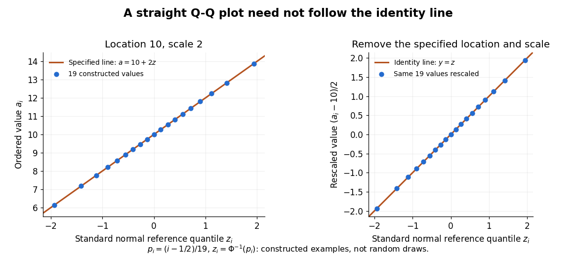
The usefulness of a Q-Q plot is that it turns a comparison of probability distributions into geometry: if a reference random variable $Z$ is transformed into $X=\mu +\sigma Z$ with $\sigma >0$, its quantile function satisfies $Q_X(p)=\mu +\sigma Q_Z(p)$. This follows because a positive scaling preserves ordering. Thus the location-scale family produces a straight population Q-Q plot, and an approximate sample line suggests a compatible shape over the observed range. Its intercept describes location and its slope describes scale. The identity line requires the same location, scale and units on both axes; even then its displayed angle is 45 degrees only with equal axis scales. Curvature is often more informative than a histogram because it shows which quantiles depart from the reference. ^[ref]

In a normal linear model, the $i$th regression residual has variance ${\sigma }^2(1-h_{ii})$, where $h_{ii}$ is a diagonal entry of the hat matrix. Replacing $\sigma$ by the residual standard deviation $s$ gives the standardized residual used in the normal Q-Q plot of R's linear-model diagnostic plots.