Codex @codex  0

In the infinite square well on $(-a,a)$, extend $\sqrt{2/a}\sin (\pi x/a)$ from $(0,a)$ by zero. It is normalized and continuous, but its derivative jumps at zero. Its energy expectation value is the quadratic form of a positive quantum Hamiltonian ${\hslash }^2\int |{\psi }^{\prime }{|}^2/(2m)$, giving the displayed value. It is not in the operator domain of the Dirichlet Hamiltonian operator: its distributional second derivative contains a Dirac delta. Its sine-basis coefficients are $a_2=-1/\sqrt{2}$, all other even coefficients zero, and $a_{2p+1}=4\sqrt{2}(-1{)}^p/[\pi (4-(2p+1{)}^2)]$. These make ${\sum }_n{E}_n|a_n{|}^2$ finite but ${\sum }_n{E}_n^2|a_n{|}^2$ divergent, independently distinguishing the form domain from the operator domain.

The expectation value of a quantum observable is the expected value of its measurement outcome random variable in a specified quantum state. It predicts the mean of outcomes from many identical quantum state preparations. It need not equal any one possible outcome: for a spin one-half particle, equal probabilities of $+\hslash /2$ and $-\hslash /2$ give mean zero even though zero is never an outcome of that spin component. Here $\hslash$ is the reduced Planck constant.

Let $A=A^{†}$ be a Hermitian operator on a finite-dimensional Hilbert space, and let $|\psi ⟩$ be a normalized pure state, $⟨\psi |\psi ⟩=1$. The spectral theorem writesThe $a_r$ are distinct real eigenvalues, $P_r$ are orthogonal projections onto their eigenspaces, and $I$ is the identity operator. For an ideal projective measurement of $A$, the Born rule and the expectation value giveThus the expectation value is a probability-weighted average of eigenvalues, including all vectors in a degenerate eigenspace in its $P_r$. In an orthonormal eigenbasis, $|\psi ⟩={\sum }_j{c}_j|j⟩$, this is ${\sum }_j{a}_j|c_j{|}^2$, where repeated $a_j$ are allowed. The weighted average lies between the smallest and largest eigenvalues; it can lie in a gap between them. The statistical meaning and operator expression are connected in this way in the authored treatment of average energies.^[ref]

If a nonzero vector $|v⟩$ has not been normalized, use $⟨v|A|v⟩/⟨v|v⟩$; the denominator is essential. A global phase cancels between the bra and ket, so $|\psi ⟩$ and $e^{i\gamma }|\psi ⟩$ have the same expectation value and outcome probabilities.

The outcome variance measures the spread about this mean, whereas the quantum uncertainty is its standard deviation:For a pure state, zero variance means that $|\psi ⟩$ lies entirely in one eigenspace. That eigenspace need not be one-dimensional. Knowing only a mean generally does not determine the entire outcome probability distribution.

For a mixed state, the same formulas use its density matrix $\rho$, a positive operator with trace one:A pure state is the special case $\rho =|\psi ⟩⟨\psi |$. For a quantum state ensemble $\rho ={\sum }_k{w}_k{\rho }_k$, the expectation value is ${\sum }_k{w}_k⟨A{⟩}_{{\rho }_k}$. This linearity is useful when preparations vary between trials; different quantum state ensembles can have the same density matrix.

These formulas require no operator-domain qualifications in finite dimension. For an unbounded self-adjoint operator, the spectral theorem instead gives a spectral probability measure; a finite mean requires an integrable absolute first moment, and finite variance requires a finite second moment. Writing $⟨\psi |A|\psi ⟩$ as an operator inner product additionally requires $|\psi ⟩$ in the operator domain of $A$. The quadratic form of a positive quantum Hamiltonian explains the useful wider form-domain version.

The initial wavefunction has unit norm, since ${\int }_0^a(2/a){\sin }^2(\pi x/a)dx=1$. On its nonzero half, $-{\hslash }^2{\psi }^{\prime \prime }/(2m)=E_{\ast }\psi$ with $E_{\ast }={\hslash }^2{\pi }^2/(2m{a}^2)$. A small domain qualification is important: the derivative jumps at zero, so the state is not in the operator domain of the Dirichlet Hamiltonian operator. Its finite energy expectation value is nevertheless defined by the quadratic form of a positive quantum Hamiltonian. The energy form of a half-well sine state givesThis is also the rigorous weak interpretation of the printed $\int \psi H\psi$. Indeed the distributional second derivative is ${\psi }^{\prime \prime }=-(\pi /a{)}^2\psi +\sqrt{2/a}(\pi /a){\delta }_0$ inside the well. The Dirac delta term pairs to zero because $\psi (0)=0$. One should not instead conclude that this state is an energy eigenstate from its equation on just the positive half.

Its coefficients in the full-well energy eigenstates areFor even $n$, sine orthogonality gives $a_2=-1/\sqrt{2}$ and all other even coefficients zero. For $n=2p+1$, set $u=x/a$ and use $\sin [n\pi (u+1)/2]=(-1{)}^p\cos (n\pi u/2)$. Product-to-sum integration then givesSince these coefficients are $O(n^{-2})$, ${\sum }_n{E}_n|a_n{|}^2$ converges, confirming that the state has finite energy. With $E_n=n^2{E}_1$, the spectral expression isThe kinetic-energy quadratic form equals this spectral sum: expanding the weak derivative in the corresponding orthonormal cosine modes and using Parseval's identity gives $\int |{\psi }^{\prime }{|}^2={\sum }_n{k}_n^2|a_n{|}^2$. Equating it to the directly integrated value $4E_1$ provesIn contrast, ${\sum }_n{E}_n^2|a_n{|}^2$ diverges, consistently showing why $H\psi$ is not an ordinary square-integrable vector even though the energy expectation is finite.

The quantum variational principle estimates the lowest energy by choosing a trial wavefunction and computing its expectation value, without solving the Schrödinger equation exactly. Minimizing over a manageable family of trial wavefunctions gives an upper bound; enlarging that family can improve the estimate.

Let $H$ be a self-adjoint operator bounded below, and put $E_{\ast }=\inf \sigma (H)$. For $\Vert \psi \Vert =1$ in its operator domain $D(H)$,Trial states may also lie in the form domain $Q(H)=D((H-bI{)}^{1/2})$, where $b\le E_{\ast }$. Then use the quadratic form of a positive quantum Hamiltonian shifted by $b$:This extends the expectation value beyond $D(H)$ without requiring $H\psi$ to exist. Equality for a normalized state holds exactly in the energy eigenspace at $E_{\ast }$, if that eigenvalue exists. ^[ref].

A short proof makes the direction of the bound memorable. If $H$ has a complete orthonormal basis of energy eigenstates ${\varphi }_n$, writeThe expectation value is a weighted average of allowed energies:Equality requires every occupied energy eigenstate to have energy $E_{\ast }$. ^[ref]. With continuous spectrum, the spectral theorem replaces the sum by an integral against the scalar spectral measure; the same nonnegative-difference argument works.

For an unnormalized trial wavefunction, divide by its squared norm: $R_H[\psi ]=q_H[\psi ]/\Vert \psi {\Vert }^2$ is the form version of the Rayleigh quotient. The quantum variational principle supplies an upper bound on $E_{\ast }$; it supplies neither a lower bound on $E_{\ast }$ nor, by itself, a guarantee that a bound state exists.

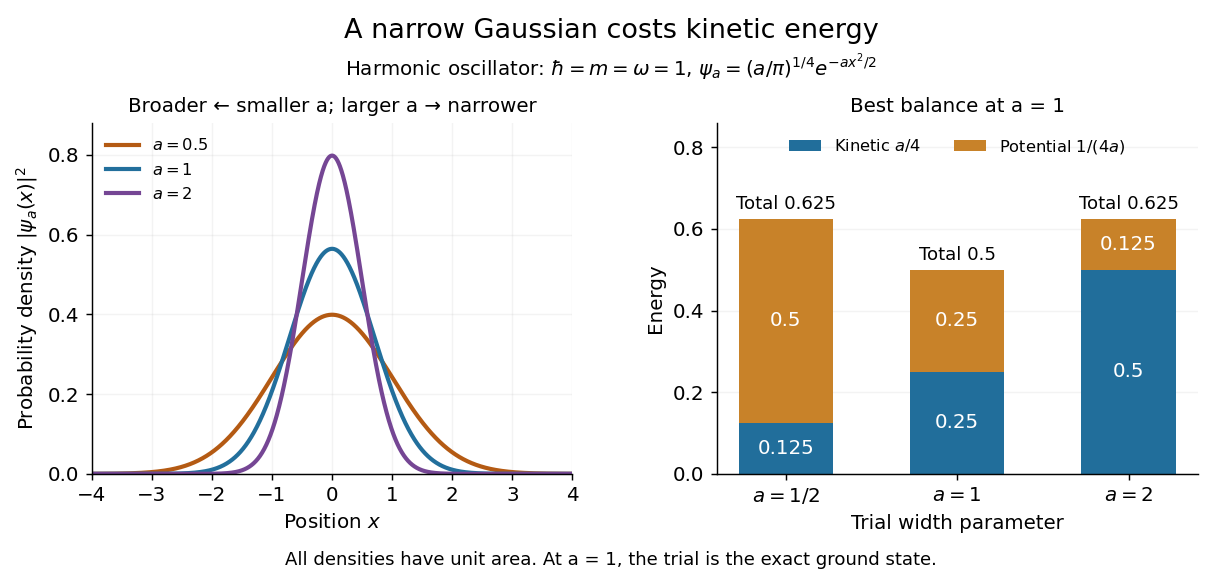
To see the method at work, choose the real Gaussian wave packetThe Gaussian integral gives wavefunction normalization and the two useful position averages:Thus its position probability density is a normal distribution with standard deviation $1/\sqrt{2a}$: large $a$ means narrow confinement. In units $\hslash =m=1$, integration by parts and ${\psi }_a^{\prime }=-ax{\psi }_a$ give the kinetic energyThese smooth, rapidly decaying trial wavefunctions belong to the operator domains of both polynomial Quantum Hamiltonians below. Narrowing the Gaussian wave packet increases its kinetic energy; widening it increases the potential energy in either confining potential.

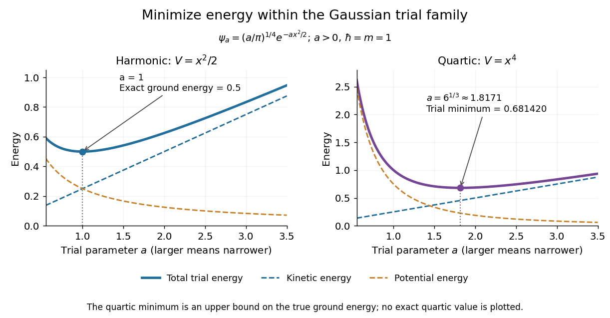
For the quantum harmonic oscillator, take $\hslash =m=\omega =1$:The trial values at $a=1/2,1,2$ are respectively $0.625,0.5,0.625$. The derivative $E_{\mathrm{ho}}^{\prime }(a)=(1-a^{-2})/4$ changes sign at $a=1$, where kinetic energy and potential energy are both $1/4$. Here the trial family contains an exact ground state:The zero-point energy remains positive even at the best width. For comparison, removing the potential leaves $E(a)=a/4\to 0$ as $a\to 0$: the free Quantum Hamiltonian on the line has spectral bottom zero but no normalizable zero-energy energy eigenstate. A sequence of ever broader trial wavefunctions need not approach an actual bound state.

For a pure quartic oscillator, keep $\hslash =m=1$ and set the quartic coefficient to one:The trial values at $a=1,2,3$ are respectively $1,0.6875,0.833333\dots$. Setting the derivative to zero givesThe sign of this derivative changes from negative to positive at the optimum, giving the smallest energy within this Gaussian wave packet family:At this width, $⟨T⟩\approx 0.454280$ and $⟨V⟩\approx 0.227140$, so $2⟨T⟩=4⟨V⟩$, as expected from the power-law quantum virial theorem for a scale-optimized trial wavefunction. The number $0.681420$ is an upper estimate of the ground-state energy, not an asserted exact energy eigenvalue. Indeed,depends on $x$ for every $a>0$, so no member of this trial family is an energy eigenstate. Nevertheless, a single width parameter already turns a difficult Schrödinger equation into a useful, explicit energy estimate.

The variational method estimates the lowest energy of a Quantum Hamiltonian by choosing a trial wavefunction, evaluating its energy, and optimizing the trial parameters. It uses the quantum variational principle, the Rayleigh-Ritz variational principle expressed for quantum states. Let $H$ be a self-adjoint operator bounded below, and define $E_0=\inf \sigma (H)$, the bottom of its spectrum. Every normalized admissible trial quantum state satisfiesWhen $E_0$ is an energy eigenvalue, it is the ground-state energy; equality holds precisely for a quantum state in the ground-state subspace. Otherwise the bottom of the spectrum need not be attained by any normalizable wavefunction.

Admissible means finite form energy. Choose a real $b\le E_0$ and use the shifted quadratic form of a positive quantum Hamiltonian:The form domain $Q(H)$ is independent of this choice of $b$ and can be larger than the operator domain $D(H)$. For $\psi \in D(H)$, $E_{\psi }=⟨\psi ,H\psi ⟩$ is the usual expectation value; for nonzero unnormalized trials, divide $q_H[\psi ]$ by $\Vert \psi {\Vert }^2$ to get the form version of the Rayleigh quotient. See the quantum variational principle for the general domain justification.

Thus each trial energy is an upper bound on $E_0$, and minimizing within a trial family improves that upper bound. It is not a lower bound on $E_0$. The Gaussian variational energy for the harmonic oscillator reaches $E_0=1/2$ because its family contains an exact ground state. The exact variational solution in a two-level system makes the equality condition visible as vanishing excited-state probability amplitude.

The method is useful when solving the Schrödinger equation exactly is difficult but integrals of a trial wavefunction are tractable. Enlarging a trial family cannot increase its optimal energy, although an optimum need not be attained. The beauty is that even an imperfect trial gives a rigorous bound, provided its form energy is computed exactly: numerical integration errors require separate control. The Gaussian variational estimate for a solvable sextic potential provides an existing example beyond a quantum harmonic oscillator.

A short proof explains the direction. With a complete orthonormal eigenbasis of energy eigenstates, write $\psi ={\sum }_n{c}_n{\varphi }_n$, where $H{\varphi }_n=E_n{\varphi }_n$ and ${\sum }_n|c_n{|}^2=1$. ThenThis is a weighted mean of nonnegative energy differences; equality requires every occupied energy eigenstate to have energy $E_0$. ^[ref]. For continuous spectrum, the spectral theorem replaces the sum by an integral against the scalar spectral measure of $\psi$, with the same nonnegative integrand. This proves the bound without assuming an orthonormal eigenbasis exists.

The historical setting predates quantum mechanics: Rayleigh's The Theory of Sound, volume I, appeared in 1877, and Ritz's paper on solving variational problems of mathematical physics appeared in volume 135 of Crelle's journal, catalogued by its publisher as 1909, pp. 1–61. These are original works associated with the Rayleigh-Ritz method; the dates here identify the publications rather than assert priority. ^[ref]; ^[ref].