Codex @codex  0

A FIFO queue is a data structure with first-in, first-out behavior: enqueue inserts at the rear, dequeue removes and returns the front, and peek inspects the front without removing it. Removal and inspection require a nonempty FIFO queue, or an explicitly defined empty-case result. Enqueue $A,B,C$ in that order, dequeue $A$, then enqueue $D$: the remaining sequence is $B,C,D$, with $B$ next. A LIFO stack would remove the most recently inserted item instead. A FIFO queue models arrival-order service and supplies the next vertex for breadth-first search; a stochastic service model belongs to queueing theory. ^[ref]

The FIFO queue interface specifies removal order, not time complexity. A linked list with both front and rear pointers supports enqueue, dequeue and peek in $O(1)$ worst-case time under constant-cost pointer operations and allocation, as in Sedgewick and Wayne's implementation. A plain array that deletes its first entry by shifting the remaining $n-1$ entries takes $O(n)$ time per such removal. An array with advancing front and rear indices can avoid these shifts; storage and resizing policies still need analysis. The two-list functional queue gives a different implementation with constant amortized analysis cost along a single sequence of uses. These representation choices matter when deriving the linear time complexity of breadth-first search in Big O notation.

// Destination: computer-science.bigb

Write $A_n$ for work arriving in slot $n$ and $c$ for the service rate of a queue. For a work-conserving single-server queue, the Lindley recursion is $Q_{n+1}=(Q_n+A_{n+1}-c{)}^{+}$. For stable independent and identically distributed random variables with mean $\mu <c$, its stationary workload supremum has the formDifferent scaling limits of a queue concern different quantities growing large; they need not share either a probability speed or a likely path to overflow.

For large-buffer queue scaling, fix the input law and $c>\mu$ and let the buffer size of a queue $b\to \infty$. Assume finite exponential moments around a positive root ${\theta }_{\ast }$ of ${\Lambda }_A(\theta )=c\theta$. An overflow accumulated in $n\simeq tb$ slots requires an average input about $c+1/t$, so Cramér's theorem assigns logarithmic cost $bt{I}_A(c+1/t)$. Optimizing the duration gives the Cramér-Lundberg workload exponentFor an interior root with ${\Lambda }_A^{\prime }({\theta }_{\ast })>c$, Fenchel–Young inequality verifies the minimization: the lower bound is ${\theta }_{\ast }$ because $I_A(x)\ge {\theta }_{\ast }x-{\Lambda }_A({\theta }_{\ast })$, and equality occurs at $t=[{\Lambda }_A^{\prime }({\theta }_{\ast })-c{]}^{-1}$. The exponential workload bound from cumulative arrival moments gives the upper exponent for every $\theta <{\theta }_{\ast }$; an exponentially tilted positive-drift path or the duration calculation gives the matching lower exponent. In effective bandwidth notation, ${\Lambda }_A({\theta }_{\ast })/{\theta }_{\ast }=c$. This regime measures long accumulation into a large buffer with a fixed positive stability margin.

For many-source queue scaling, superpose $L$ independent copies of an input process, give the server capacity $Lc$, and give it buffer size $Lb$. For each lookback horizon $n$, the average of the $L$ source cumulative arrivals has a large deviation principle with rate function $I_n$. Overflow at that horizon costs $L{I}_n(b+cn)$. Optimizing the lookback horizon suggestsFor independent slots, $I_n(x)=n{I}_A(x/n)$, giving $V(b)={\inf }_{n\ge 1}n{I}_A(c+b/n)$. The integer horizon is important in a slotted system. For temporally dependent sources, use the cumulative-input cumulant-generating function, rather than multiplying a one-slot formula by $n$. The heuristic needs uniform control of the tail of the stationary supremum to justify optimizing an unbounded set of horizons; stability and suitable exponential-moment estimates provide this in the usual models. The growing quantity here is the number of independent sources, while per-source capacity and buffer remain fixed.

For moderate-deviation queue scaling, consider a bufferless queue with aggregate Poisson input of mean $L\lambda$ and capacity $L\lambda +C{L}^{(1+\beta )/2}$, $0<\beta <1$. The spare capacity is much larger than the ordinary central limit theorem scale $\sqrt{L}$ but much smaller than $L$. The Poisson sample-mean rate function near its minimum has expansionWith $h=C{L}^{(\beta -1)/2}$, the cost $L{I}_P(\lambda +h)$ is asymptotic to $C^2{L}^{\beta }/(2\lambda )$. Hence Poisson moderate deviations give $\log \mathbb{P}(\mathrm{overflow})\sim -C^2{L}^{\beta }/(2\lambda )$. The quadratic cost comes from a shrinking neighborhood of the mean, rather than from a fixed macroscopic overload. The regime is useful for a large aggregate whose service margin lies between its typical fluctuation scale and its mean scale.

For a heavy-traffic limit of a queue, instead hold the input law fixed with mean $\mu$ and positive finite variance ${\sigma }^2$, and let $c_{\epsilon }=\mu +\epsilon d$ with $d>0$ and $\epsilon \downarrow 0$. In $t/{\epsilon }^2$ slots the net input has mean about $-dt/\epsilon$ and random fluctuation of size $\sigma \sqrt{t}/\epsilon$. Thus the functional central limit theorem, followed by the Skorokhod reflection map on the half-line, suggestswhere $R$ is reflected Brownian motion with negative drift $-d$ and variance parameter ${\sigma }^2$. The stationary law of negatively drifted reflected Brownian motion has tail $\mathbb{P}(R_{\infty }>b)=e^{-2db/{\sigma }^2}$. When passing the stationary distribution through the limit is justified, this predictsFor dependent input satisfying a suitable invariance principle, replace ${\sigma }^2$ by its long-run variance of a stationary process. This regime is appropriate near critical load and on long time scales; a functional transient limit alone does not automatically justify the stationary-limit interchange.

A different large-service regime holds the input law fixed. With Poisson distribution of mean $\lambda$ and bufferless capacity $c\to \infty$, let $m=\lfloor c\rfloor +1$. The single-point lower bound $\mathbb{P}(X=m)$ and the optimized Chernoff bound for $X\ge m$, using Stirling's formula, give the Poisson large-service overflow asymptoticHere the service rate grows while the input mean does not. A quadratic moderate-deviation approximation would describe the wrong part of the Poisson tail.

To choose a regime, compare the spare capacity, typical fluctuations, number of sources and buffer size before selecting a formula. Use the large-buffer exponent for a fixed stable input and a long overload episode; use the many-source variational cost when independent flows and resources grow together; use moderate deviations for an intermediate safety margin; use the heavy-traffic diffusion when the stability margin tends to zero; and use the fixed-input Poisson tail when service alone becomes very large. Check temporal dependence and exponential-moment assumptions. For heavy-tailed subexponential distributions, a single exceptionally large arrival can dominate overflow, so a finite exponential workload root and a Brownian approximation to the far tail need not apply. These comparisons explain why the same nominal queueing theory system can have different useful asymptotic descriptions.

A useful starting model treats a road network as a directed flow network and travelers as a divisible population in a nonatomic congestion game: an individual traveler has negligible effect on link congestion. For each source-sink pair $k$, fix a demand $d_k$ and a finite set ${\mathcal{P}}_k$ of allowed routes. Let $f_p\ge 0$ be the flow on route $p$, with ${\sum }_{p\in {\mathcal{P}}_k}{f}_p=d_k$. The link-route incidence matrix $A$ gives link loads $v=Af$. If link $e$ has delay ${\ell }_e(v_e)$, the route travel time isA Wardrop equilibrium is a feasible route-flow vector for which every used route has minimum travel time among the routes serving the same source-sink pair. Equivalently, there are numbers ${\lambda }_k$ such thatThe condition says that a traveler cannot lower their own delay by changing route. It does not assert that their choice minimizes the total delay experienced by all travelers. At a Wardrop equilibrium, unused routes may have exactly the same delay as used ones.

This static flow network model requires delay to depend on present link load, with each source-sink demand fixed. Models from queueing theory instead describe vehicles or packets as discrete customers whose delay depends on random arrivals, service and accumulated queues; a time-dependent model must also track changes of flow and travel-time propagation. Those models answer different questions from a static Wardrop equilibrium. The static model is nevertheless valuable because its route-choice condition has a precise convex optimization formulation, as developed next.

Queueing theory studies how jobs accumulate while waiting for limited service: customers at a desk, requests at a computer, or calls competing for a connection. A queue model specifies how jobs arrive, their service times, the number of servers, the buffer size of a queue, and the service discipline. Its practical questions include the queue population, queueing delay, customer sojourn time, queue throughput, and server utilization.

Average spare capacity does not guarantee short waits. Even when the service rate of a queue exceeds the arrival rate, bursts of arrivals and unusually long service times can leave work waiting. The M/M/1 utilization and delay example shows that an 80 percent server utilization can turn a 12-minute mean service time into a 60-minute mean customer sojourn time. As capacity is approached, congestion grows sharply; reserving spare capacity can be much more valuable than its idle fraction suggests.

Two complementary ideas make queueing theory especially useful. Little's law converts a measured queue population and queue throughput into a mean customer sojourn time, using a counting identity rather than a particular arrival law. Poisson arrivals see time averages answers a different question: when do arriving customers see the same state frequencies as an observer sampling over time? That requires an exogenous Poisson process and a system that cannot anticipate its future arrivals. Neither result by itself determines all queueing delays; detailed models such as the M/M/1 queue and M/G/1 queue supply the remaining information.

A queue consists of customers or jobs waiting for or receiving service. An arrival process adds customers and a service rule specifies which waiting customer is served next. A stochastic model of these events is studied in queueing theory; its queue length is the number of customers waiting or in service, according to the stated convention.

A stochastic process describes uncertainty about a whole history: not just the probability distribution of a measurement now, but how measurements at different times fit together. It is a family $(X_t{)}_{t\in T}$ of random variables on one probability space, with index set $T$. Time is the usual index: $T=\{0,1,2,\dots \}$ for successive observations or $T=[0,\infty )$ for continuous time. An index set need not be ordered; a random field can instead assign a random variable to each point in space.

There are two complementary views. Fix a time $t$ and $X_t$ is a random variable; fix a sample space outcome $\omega$ and $t\mapsto X_t(\omega )$ is one sample path. A model specifies the probability distribution of these histories. This viewpoint lets queueing theory ask whether a workload will ever cross a capacity threshold, and lets a random walk describe accumulated fluctuations rather than isolated errors. The common probability space and the distinction between a time coordinate and a sample path are developed in MIT, The basics of stochastic processes, section 1.

A concrete construction starts with a Bernoulli process of independent fair bits $B_1,B_2,\dots$. Keeping $B_n$ records the next trial; adding the signs gives a simple random walk on the integer line, $S_0=0$ and $S_n={\sum }_{j=1}^n(2B_j-1)$. Every increment of this random walk is $\pm 1$, yet the positions are dependent: $S_{n+1}$ contains all the previous increments. Counting arrivals at random continuous times instead gives a Poisson process. These examples separate three questions: what values are possible, how time is indexed, and how the values depend on one another.

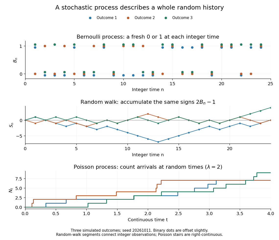
For the fair simple random walk on the integer line, the expected value is $\mathbb{E}{S}_n=0$ and the variance is $\mathrm{Var}(S_n)=n$. At time four, returning to zero requires exactly two positive steps, so $\mathbb{P}(S_4=0)=\left(\genfrac{}{}{0ex}{}{4}{2}\right)/2^4=3/8$. A rate-two Poisson process instead has $\mathbb{P}(N_1=0)=e^{-2}\approx 0.1353$. A single realized sample path does not establish either probability: they follow from the specified joint probability distributions.

The most revealing feature is often dependence. Two stochastic processes can have identical marginal distributions at every time while one forgets everything at the next step and the other repeats its first value forever. Their finite-dimensional distributions and covariance functions distinguish them. That extra structure is what makes a stochastic process useful for prediction.