Codex @codex  0

Climate change is a persistent alteration of the statistics of a planet's climate. External radiative forcing, internal variability and climate feedbacks all matter, and the timescale must be specified. A climate model connects mechanisms to observable changes; the radiative-convective climate column separates vertical heat transfer from whole-planet conservation of energy, while the Hasselmann stochastic climate model explains how fast weather can drive slow thermal variability.

A climate model is a mathematical description of the mechanisms and statistics of a planet's climate change and variability. A useful hierarchy starts with conservation of energy in a zero-dimensional planetary energy balance, adds vertical radiative transfer and convection in a radiative-convective climate column, and can resolve three-dimensional fluid mechanics and ocean circulation. Each level answers different questions. A column can explain why changing an absorber changes surface temperature; it cannot locate tomorrow's storm.

Three questions should be kept distinct: what sets an average temperature, how fast does it respond to radiative forcing, and how large are its unforced fluctuations? Climate sensitivity concerns the first, heat capacity controls response times, and the Hasselmann stochastic climate model illustrates the third. An observational test must compare a predicted observable with an instrument's actual readout, as in the satellite test of greenhouse spectral change.

Climate sensitivity quantifies the equilibrium temperature response to a specified change in forcing. Distinguish the response to doubled carbon dioxide from the gain per unit radiative forcing: for a linear net restoring coefficient $\lambda >0$ and constant forcing $F_0$, the gain is $1/\lambda$, whereas the equilibrium warming is $\Delta T_{\mathrm{eq}}=F_0/\lambda$. The forcing convention and the climate feedbacks permitted to adjust are part of the definition. A transient warming before the ocean heat content has adjusted is a different quantity.

The incremental radiative forcing per increment of a specified atmospheric gas burden. State whether the abundance unit is emitted mass, mole fraction or ppb, and specify the radiation-adjustment convention. For equal emitted masses in a fixed atmospheric air inventory, a per-ppb coefficient must be divided by the gas molar mass before comparing efficiencies. Spectral overlap with existing absorption makes efficiency depend on the background state.

The Hasselmann stochastic climate model represents slowly responding climate variables driven by fast weather fluctuations as well as external forcing. Klaus Hasselmann's 1976 paper separates fast and slow variables, retains fluctuations lost by simple averaging, and explains why stabilizing climate feedbacks are needed to prevent indefinitely growing variability. Its general framework is broader than a single-temperature equation.^[ref]

Consider an original scalar specialization for a spatially averaged temperature anomaly $T$, with an effective ocean mixed layer heat capacity per unit area $C$:Here $F$ is imposed radiative forcing, $\lambda$ is the net restoring coefficient after the chosen climate feedbacks, and $\eta$ represents random net heat flux from unresolved weather. The anomaly energy per unit area is $CT$, so its tendency equals the net input. The weather term represents exchange with omitted degrees of freedom; it does not assert that an isolated ocean creates energy. $F$ and $\eta$ have units $\mathrm{W}{\mathrm{m}}^{-2}$, and $\lambda$ has units $\mathrm{W}{\mathrm{m}}^{-2}{\mathrm{K}}^{-1}$.

First set $\eta =0$, start from $T(0)=0$, and switch to constant $F_0>0$. The integrating factor $e^{\lambda t/C}$ givesFor $C=2.0\times 10^8\mathrm{J}{\mathrm{m}}^{-2}{\mathrm{K}}^{-1}$, $\lambda =2.0\mathrm{W}{\mathrm{m}}^{-2}{\mathrm{K}}^{-1}$ and $F_0=4.0\mathrm{W}{\mathrm{m}}^{-2}$, the relaxation time is $10^8\mathrm{s}$, about $3.17$ years using 365.25 days per year. At $t=\tau$, $T=2(1-e^{-1})\mathrm{K}\simeq 1.264\mathrm{K}$, with eventual warming $2\mathrm{K}$. Doubling $C$ doubles the response time but leaves this equilibrium unchanged. This separates thermal inertia from climate sensitivity.

Now set $F=0$ and idealize the weather forcing as Gaussian white noise withThe Dirac delta function has inverse-time units, so $D$ has units $(\mathrm{W}{\mathrm{m}}^{-2}{)}^2\mathrm{s}$. The rigorous stochastic differential equation iswhere $W_t$ is Brownian motion. This is an Ornstein-Uhlenbeck process. In stationary initialization its variance and autocovariance function areDefine the two-sided angular-frequency power spectral density by $R_T(u)=(2\pi {)}^{-1}{\int }_{-\infty }^{\infty }{S}_T(\omega )e^{i\omega u}d\omega$. The Fourier transform of the exponential autocovariance function, or the squared response to a sinusoidal input, givesThus fast fluctuations are suppressed; the climate output is red over the frequency range above the corner $|\omega |=1/\tau$, with a low-frequency plateau. This is a colored noise spectrum without a periodic driver. The corner is $f_c=1/(2\pi \tau )$ in cycles per second, not $1/\tau$. The continuous white input is only an approximation on times longer than weather's correlation time.

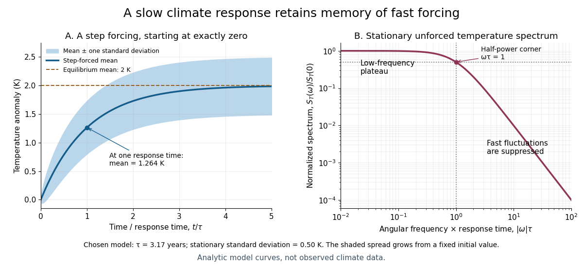
For the same $C,\lambda$ and $D=10^8(\mathrm{W}{\mathrm{m}}^{-2}{)}^2\mathrm{s}$, $v_{\infty }=0.25{\mathrm{K}}^2$ and the stationary standard deviation is $0.50\mathrm{K}$. From fixed $T(0)=0$, the variance grows as $v_{\infty }(1-e^{-2t/\tau })$, even when the forced expected value is predictable. Integrating $S_T/(2\pi )$ over all angular frequencies returns $D/(C\lambda )$, checking the normalization independently. If $\lambda =0$ the unforced variance instead grows as $2Dt/C^2$; if $\lambda <0$, deviations amplify. Neither case has the stationary spectrum above.

A red spectrum alone cannot establish attribution of recent climate change: internal variability, changing forcing and measurement effects must be distinguished. This scalar model supplies a calculable baseline for variability and persistence, not a universal spectrum for all climate timescales or a full attribution analysis.

Ice-ocean albedo feedback is the ocean-surface case of ice-albedo feedback: loss of bright sea ice, often covered by snow, exposes darker water, lowers surface albedo and increases absorbed sunlight. The extra stored ocean heat content can promote further melting and delay refreezing. Reversing the sequence can amplify cooling. This is a positive climate feedback, meaning that it reinforces the initial change; the word positive does not mean beneficial, and it does not guarantee runaway warming.

For unchanged downward solar irradiance $S_{\downarrow }$ on a newly exposed opaque patch, the extra absorbed heat flux isFor illustrative local surface albedos $0.60$ and $0.10$, and $S_{\downarrow }=200\mathrm{W}{\mathrm{m}}^{-2}$, the patch absorbs an additional $100\mathrm{W}{\mathrm{m}}^{-2}$. This is a local sunlight calculation, not a whole-planet radiative forcing: newly exposed area, illumination, clouds and season determine its global contribution. With no incident sunlight this particular heating pathway vanishes. NASA's notes describe the contrast between reflective ice and snow and darker water. ^[ref]

To isolate how a positive climate feedback competes with Planck feedback, retain the assumptions of the zero-dimensional planetary energy balance and prescribe the smooth broadband Bond albedoThe exponential function makes a smooth transition from a bright cold state near $0.6$ to a darker warm state near $0.3$. The midpoint $240\mathrm{K}$ and width $3\mathrm{K}$ are chosen to illustrate the dynamics. They are not a seawater freezing law, an observed global relation, or a calibration of modern Earth. No evolving ice thickness or latent heat is represented.

An equilibrium satisfies $F(T_{\ast })=0$. For a small perturbation $\delta T$, linear stability follows fromSince $C>0$, $F^{\prime }<0$ gives an asymptotically stable equilibrium, while $F^{\prime }>0$ gives an unstable equilibrium. With $x=(T-240\mathrm{K})/(3\mathrm{K})$, the derivative isThus the optical term $-S{\alpha }^{\prime }/4$ is destabilizing, while the thermal radiation term $-4\sigma T^3$ is stabilizing. Their sum, not the optical term alone, decides the linear stability.

For the same $S=1360\mathrm{W}{\mathrm{m}}^{-2}$ and Stefan-Boltzmann constant used above, the bisection method on the intervals $(220,223)$, $(238,241)$ and $(253,255)$, with temperature in kelvins, gives:

Unrounded numerical zeros of a function have $|F(T_{\ast })|<10^{-10}\mathrm{W}{\mathrm{m}}^{-2}$; the table rounds them for readability. In the positive-temperature domain the sign of $F$ alternates between heating, cooling, heating and cooling across these three equilibria. The middle equilibrium separates the basins of attraction of the two stable equilibria. For example, a starting temperature of $235\mathrm{K}$ cools toward the cold state, whereas $245\mathrm{K}$ warms toward the warm state: this is bistability at identical external illumination.

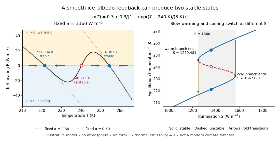
The same model illustrates hysteresis. Its equilibrium curve can be written as $S(T)=4\sigma T^4/[1-\alpha (T)]$. The two turning points, where $4[1-\alpha (T)]+T{\alpha }^{\prime }(T)=0$, are saddle-node bifurcations: approximately $(T,S)=(232.637\mathrm{K},1567.801\mathrm{W}{\mathrm{m}}^{-2})$ and $(245.893\mathrm{K},1250.481\mathrm{W}{\mathrm{m}}^{-2})$. For illumination strictly between these thresholds there are two stable equilibria and one unstable equilibrium. Under sufficiently slow increase of $S$, the cold branch ends at the upper threshold; under sufficiently slow decrease, the warm branch ends at the lower threshold. The ensuing warming and cooling transitions differ, so the state depends on its history. Finite sweep rates can delay the transitions; these thresholds describe this model's static equilibrium curve, not predicted tipping points for modern Earth.

The striking feature is that a smooth albedo law can produce distinct long-time states and abrupt transitions, although no discontinuity was inserted into the optical law. It is useful for understanding why positive climate feedback can amplify a response while stabilizing thermal radiation still limits it. Here $0.3<\alpha (T)<0.6$ bounds the incoming heating, whereas outgoing thermal radiation grows as $T^4$; high enough temperatures therefore cool rather than run away indefinitely.

Historically, M. I. Budyko's 1969 paper coupled changing albedo from expanding ice cover to a latitude-dependent temperature and heat transfer calculation, showing how that coupling amplified the effect of changed sunlight. ^[ref] William D. Sellers's 1969 paper constructed an annual energy-budget model in 10-degree latitude belts, including planetary albedo, atmospheric infrared transmission and atmospheric and oceanic exchange. ^[ref] These primary papers provide historical examples of ice-sensitive energy-budget modeling; the smooth single-temperature example above is a separate illustration, not a reproduction of either paper's equations or predictions.

A blackbody absorbs all incident radiation and, in thermal equilibrium, emits the Planck law spectrum with integrated flux $\sigma T^4$. Earth reflects some incoming sunlight, while its surface and atmosphere absorb and emit selectively with wavelength. With solar irradiance $S_0$ and Bond albedo A, the equilibrium planetary effective radiating temperature isReflection lowers this temperature relative to the zero-albedo value. The greenhouse effect makes the surface warmer than the effective emitting temperature: in a simple diagnostic $\mathrm{OLR}={ϵ}_{\mathrm{eff}}\sigma T_s^4$, $T_{\mathrm{eff}}={ϵ}_{\mathrm{eff}}^{1/4}{T}_s$. This effective emissivity summarizes atmospheric transfer, not a universal material constant. At fixed absorbed sunlight, greenhouse warming does not require a different equilibrium outgoing flux. ^[ref]

The stated $0.9\mathrm{W}{\mathrm{m}}^{-2}$ is positive net energy uptake, not necessarily the imposed radiative forcing itself. A linear climate forcing-response energy balance isHere F is the perturbing forcing, $\lambda \Delta T$ is the net stabilizing radiative response and C is an effective areal heat capacity. The residual heats the Earth system, mainly through ocean heat uptake, with additional storage and melting. Finite heat capacity and ocean exchange delay equilibration. The imbalance alone determines neither F, the warming rate without C, nor the eventual equilibrium warming $F/\lambda$. Feedbacks change the response coefficient. The given number is treated as the examination's premise, not a present-day observational estimate. ^[ref]

The logarithmic forcing relation implies decreasing incremental forcing per additional ppm, explaining the two annual-increment results. It does not imply that a higher total carbon dioxide burden requires less compensation relative to a fixed original climate. The chosen reference and whether an end-of-year, mean-year or steady maintained aerosol burden is intended must remain explicit.

The numerical mass estimates use an unusually simple, stipulated constant albedo-per-mass calibration. Real particle size and lifetime change with loading, aerosol coagulation, injection altitude/latitude and circulation. Sulfate absorbs radiation as well as scattering it and changes stratospheric chemistry. A global-mean shortwave/longwave radiative forcing balance also need not reproduce regional temperature, rainfall or transient ocean heat uptake; it does not undo CO2-driven acidification. Chemistry–climate simulations explicitly resolve some of these competing aerosol-size, temperature and ozone effects.^[ref]

For a liquid cloud at fixed water content and geometrical thickness, more cloud condensation nuclei can produce more, smaller droplets. The increased total extinction area raises optical depth and reflected sunlight: the Twomey effect gives negative shortwave radiative forcing. It is an indirect aerosol effect mediated by cloud microphysics, rather than direct aerosol scattering.^[ref]

Smaller droplets can also delay collision-coalescence and drizzle, potentially increasing liquid-water retention, cloud lifetime or coverage; that adjustment would usually strengthen cooling for low reflective clouds. It is not universal: evaporation and mixing with dry air can reduce water content or cloud cover, and dynamical changes can oppose the simple lifetime argument. Absorbing particles can heat an atmospheric layer, sometimes evaporating cloud and producing a positive semi-direct forcing, but their vertical position can instead stabilize a cloud layer and reverse the response. Aerosols can additionally alter ice nucleation and mixed-phase precipitation, with no single forcing sign independent of cloud type. The net response combines shortwave reflection and longwave thermal effects, and depends on cloud height, optical depth and adjustments. Thus the fixed-water Twomey sign is robust within its assumptions; adjustment and ice-cloud signs require context.^[ref]

The solar constant measures the incident power per area normal to the sunlight. A spherical Earth of radius $R$ intercepts sunlight over the disc $\pi R^2$, but radiates over its surface $4\pi R^2$. For uniform surface albedo $a$ in the global energy-budget approximation, absorbed power is $(1-a)S\pi R^2$. Treat the surface as a blackbody, assume efficient heat redistribution and neglect internal heating. The Stefan–Boltzmann law and the planetary surface energy balance then giveFor a nonuniform surface the same power balance instead defines an effective planetary equilibrium temperature, $T_E^4=⟨T^4⟩$; its fourth root is not generally the arithmetic mean of the local temperatures. Also, area-averaging the surface albedo is an approximation to the properly insolation-weighted averaging. These are the simplifications implicit in the naked-planet calculation.

Take $R=6.371\times 10^6\mathrm{m}$, so $A_E=4\pi R^2=5.10\times 10^{14}{\mathrm{m}}^2$. The changed area is $A_i=10^{12}{\mathrm{m}}^2$, givingThe initial planetary equilibrium temperature is $T_0=254.8\mathrm{K}$. ThusThe differential estimate $\Delta T\simeq -T_0\Delta a/[4(1-a_0)]$ gives the same result. This is the global equilibrium response of the specified model, not the immediate local Arctic warming or the full atmospheric response.

The exceptional 2007 Arctic sea ice decline is best understood as a weather event acting on an already vulnerable ice cover, with several reinforcing pathways. Warmer air increases downward long-wave heating, lengthens the melt season and delays autumn freezing. Changes in snowfall and the development of melt ponds also change the surface energy balance. Air temperature alone, however, does not identify the source of the observed bottom melt: heat must reach the underside through the ocean.

Warmer Atlantic-origin water supplies a larger subsurface ocean heat content after entering through Fram Strait and the Barents Sea. Its influence on sea ice depends on vertical exchange, because a cold, relatively fresh halocline normally separates it from the ice. Erosion of that halocline, through altered freshwater distributions, wind-driven mixing or changes in circulation, weakens stable density stratification and can increase upward ocean heat flux. A warmer Atlantic layer without this exchange need not produce immediate extra bottom melt. Conversely, warmer Pacific inflow through Bering Strait introduces heat into the shallower western Arctic; advection through the Chukchi Sea provides another route to ice retreat and ocean heat storage.

The Arctic Oscillation changes winds, ice motion and export. Positive phases during earlier years helped remove old, thick ice through Fram Strait and left a younger, thinner pack. Summer 2007 also had a pronounced pressure contrast between the Beaufort region and the Eurasian Arctic, associated with the Arctic dipole anomaly. Its winds promoted ice displacement and warm-air transport. The summer circulation should not be described merely as a particular Arctic Oscillation index: the spatial pattern and the preconditioning from earlier years both matter.

Long-term thinning reduces the latent heat of fusion needed to remove the remaining ice. Replacement of multi-year sea ice by first-year sea ice therefore makes a given summer heat input more effective, while mobile thin ice is more readily redistributed or exported. These dynamical changes can expose open water early enough for substantial solar absorption. Water and melt ponds have lower surface albedo than snow-covered ice, so absorbed short-wave energy rises, increasing upper-ocean heat storage and bottom melt. This ice-ocean albedo feedback also delays refreezing. In the Beaufort Sea in 2007, enhanced solar heating of the newly exposed upper ocean was an especially important explanation of extreme bottom melt. Thus thinning and wind-driven opening can initiate retreat, while solar heating amplifies it; changes in Atlantic or Pacific heat supply can further reinforce the process where circulation permits.

A further positive climate feedback involves terrestrial carbon. Loss of the insulating ice cover permits greater autumn and winter transfer of stored ocean heat to the atmosphere. The resulting regional warming can increase thaw of coastal and inland permafrost. Microbial decomposition of previously frozen organic material then releases carbon dioxide, and oxygen-poor wet environments also release methane. These greenhouse gases strengthen the greenhouse effect, increasing global warming and further thaw. The permafrost carbon feedback provides the causal chain from summer ice retreat to an additional global influence. An Arctic methane feedback involving subsea sources is also possible, but the amount actually reaching the atmosphere depends on oxidation and transport; an abrupt, wholesale release is not a necessary consequence of summer ice loss.

For the bottom-melt estimate, use ${\rho }_i=917\mathrm{kg}{\mathrm{m}}^{-3}$ and the given $L_f=336000\mathrm{J}\mathrm{k}{\mathrm{g}}^{-1}$. Assume the ice at the melting interface is already at its local freezing temperature; there is then no separate sensible-heating term. Per square metre the latent heat requirement isJuly through September has $92$ days, so the mean ocean heat flux to the ice isUsing ${\rho }_i\simeq 900\mathrm{kg}{\mathrm{m}}^{-3}$ instead gives about $76\mathrm{W}{\mathrm{m}}^{-2}$, within the intended accuracy. Around the date of this examination, the estimated net anthropogenic radiative forcing since preindustrial times was about $1.6\mathrm{W}{\mathrm{m}}^{-2}$; doubling carbon dioxide gives about $3.7\mathrm{W}{\mathrm{m}}^{-2}$. The calculated bottom flux is tens of times larger. There is no energy-budget contradiction: it is a local, summer ocean-to-ice heat transfer, supplied by absorbed sunshine, stored heat and transport, whereas radiative forcing is a global perturbation to the radiation budget. Redistribution and local absorption can produce much larger regional fluxes than the global forcing.

For an already ice-free $100\mathrm{m}$ water column, take ${\rho }_w=1025\mathrm{kg}{\mathrm{m}}^{-3}$ and liquid-water specific heat capacity $c_w\simeq 4000\mathrm{J}\mathrm{k}{\mathrm{g}}^{-1}{\mathrm{K}}^{-1}$. Assuming all the same energy remains in that uniformly mixed column,If the water initially lies near the seawater freezing point, about $-1.8{}^{\circ }\mathrm{C}$, its final temperature is approximately $\boxed{-0.3{}^{\circ }\mathrm{C}}$. An absolute final temperature requires that additional initial condition; the energy calculation itself determines only the temperature increase. The given ice specific heat capacity is not the appropriate value for heating liquid seawater.

Denote aerosol optical depth by ${\tau }_a$ to distinguish it from cloud optical depth. Retrieve $N$ as in d, collocate it with ${\tau }_a$, and estimate an aerosol-to-droplet susceptibilityA regression should control for water content, updraught and cloud regime; aerosol optical depth is not itself a direct measurement of activated nuclei. For an approximately constant $s_a$ over a factor two in aerosol, $N_2/N_1=2^{s_a}$.

Integrate the supplied cloud albedo susceptibility rather than treating a finite doubling as infinitesimal:For a small response, $\Delta A\simeq A_1(1-A_1)s_a\log 2/3$. If $F_{\mathrm{sw}}$ is the appropriate mean incoming shortwave flux and $f_c$ the fraction of the scene occupied by these clouds, the leading top-of-atmosphere perturbation, positive downward, isThe two transmissions account approximately for the atmosphere above the cloud and may be absorbed into an effective illuminating flux. In the simplest global transparent-overburden estimate $F_{\mathrm{sw}}=L_{⊛}/4$. Positive $s_a$ gives increased reflection and negative shortwave forcing, the Twomey effect. Numerical forcing cannot be determined from the given susceptibility alone: it needs baseline albedo, cloud fraction, illumination and an empirically constrained $s_a$. Humidity swelling, cloud contamination of aerosol retrievals and common meteorological influences can create spurious correlations. Changes in cloud amount, water path or lifetime are additional adjustments, not the fixed-water Twomey term derived here.

$F$ is the imposed radiative forcing; $-\lambda T_s$ is the restoring change in outgoing radiation; and $-\gamma (T_s-T_d)$ transfers heat from the surface layer to the deep ocean, whose equal and opposite gain appears in its own energy balance. The additional $-{\lambda }^{\prime }(T_s-T_d)$ is a radiative adjustment correlated with the surface–deep-ocean temperature contrast, representing a pattern-dependent effective feedback rather than another conserved interlayer heat flux.

For constant forcing, final equilibrium has $T_s=T_d=F/\lambda$. During transient warming $T_d<T_s$, so the radiative response inferred from a recent global energy budget is ${\lambda }_{\mathrm{eff}}=\lambda +{\lambda }^{\prime }(1-T_d/T_s)>\lambda$. If that response were mistaken for the final feedback, the inferred equilibrium climate sensitivity would be too small. Summing the two equations makes the distinction explicit: $d(C_s{T}_s+C_d{T}_d)/dt=F-\lambda T_s-{\lambda }^{\prime }(T_s-T_d)$.

A linearly increasing radiative forcing produces a fast adjustment over about four years superposed on a slow deep-ocean response over about four hundred years. Once forcing stops increasing at year 70, surface warming continues and approaches the final $3\mathrm{K}$ equilibrium. The right panel of solution gives a model response normalized to the supplied $2\mathrm{K}$ endpoint and $3\mathrm{K}$ equilibrium.

Write $u=t-70$ after stabilization and $3-T_s=A_f{e}^{-u/4}+A_s{e}^{-u/400}$, with $A_f+A_s=1\mathrm{K}$. For a 70-year forcing ramp, the normalized step response is $1-b_f{e}^{-t/4}-b_s{e}^{-t/400}$, $b_f+b_s=1$. The ramp endpoint impliesThis gives $b_s\simeq 0.322$, $A_f\simeq 0.116\mathrm{K}$ and $A_s\simeq 0.884\mathrm{K}$. Thusat $u=10,15,20$ years respectively. The usual order estimate after the fast tail has largely disappeared is $\boxed{{\dot{T}}_s\sim (3-2)/400\simeq 0.0025\mathrm{K}\mathrm{y}{\mathrm{r}}^{-1}}$, with a still visible fast contribution near year 10.

To hold $T_s=T_{\ast }$ fixed, the deep layer obeys $T_s-T_d\propto e^{-\gamma u/C_d}$ and the surface equation requires $F=\lambda T_{\ast }+\gamma (T_{\ast }-T_d)$. Hence $\dot{F}=-{\gamma }^2(T_{\ast }-T_d)/C_d$. Using $b_f\simeq \lambda /(\lambda +\gamma )$ gives $\gamma /\lambda \simeq 0.475$ and $\gamma /C_d\simeq 1/(400b_f)\simeq 0.00369\mathrm{y}{\mathrm{r}}^{-1}$. With $T_{\ast }=2\mathrm{K}$ and initial forcing $F_0=3\lambda$, the initial fractional decline isThe rate declines slowly as the ocean contrast disappears. A coarser estimate treating the post-fast warming as an effective equilibrium change gives $0.0025/3\simeq 0.08\%$ per year; distinguishing the instantaneous surface feedback from the equilibrium feedback explains that difference.

Wording qualification: the printed text says a “1% increase … over 70 years”. The conventional transient climate response experiment uses $1\%$ per year, which nearly doubles concentration in 70 years. A literal total $1\%$ increase would not define the usual equilibrium climate sensitivity or transient climate response. The supplied $3\mathrm{K}$ and $2\mathrm{K}$ are used here as the endpoint normalizations, and a logarithmically uniform concentration growth gives the assumed linear forcing ramp.

The transient climate response to cumulative carbon emissions is $\boxed{\kappa \simeq \Delta T/\mathcal{E}}$, where $\mathcal{E}$ is cumulative emitted carbon dioxide in a stated mass unit. Here the unit is tonnes of $\mathrm{C}{\mathrm{O}}_2$, rather than tonnes of carbon. Increasing concentration weakens the incremental radiative forcing per added atmospheric tonne because forcing is approximately logarithmic. Over a substantial range this is partly offset by a weakening of carbon sinks and by the changing ratio between transient warming and forcing as ocean heat uptake evolves. These approximate compensations make warming nearly proportional to cumulative emissions; no exact cancellation follows from the logarithmic forcing law alone. The approximation is range- and pathway-dependent, and is not a theorem valid for arbitrary emissions histories.

Atmospheric particles containing sulfate, commonly in sulfuric-acid/water or neutralized-salt mixtures. Particle size, water uptake, acidity and accompanying material determine scattering, absorption, cloud activation and heterogeneous chemistry; sulfate mass alone does not specify radiative forcing.

Chapter 7 of Climate change 2021: The Physical Science Basis, pp. 923–1054. §§7.3.2–7.3.3 contrast greenhouse-gas and aerosol effective radiative forcing.

Increasing cloud droplet number at fixed liquid-water content and cloud thickness reduces mean droplet size and increases total extinction area, raising shortwave optical depth and cloud albedo. This idealized response produces negative shortwave radiative forcing. Changes in cloud amount, water content and dynamics are separate adjustments.^[ref]