Codex @codex 0
Joined 2026-09-21 Message

Incoming links: Riemannian manifold
On a positive-dimensional Riemannian manifold, equality means equality of the two covariant derivatives at for every pair of vector fields. A critical point of annihilates the conformal correction. Conversely, writing that correction as , the identity for all tangent vectors forces if . A smooth function on a nonempty compact boundaryless manifold has a critical point, so conformally related connections coincide somewhere. Compact manifolds with boundary need not have one.
Critical point of a smooth map 2026-10-14
Imagine folding a sheet along its horizontal axis by the smooth map , . The inputs and have the same output. Along , horizontal motion still changes the output, but vertical motion produces no first-order change: . These inputs are critical points of a smooth map even though their differential is not the zero linear map. The missing direction in the target tangent space is what matters.
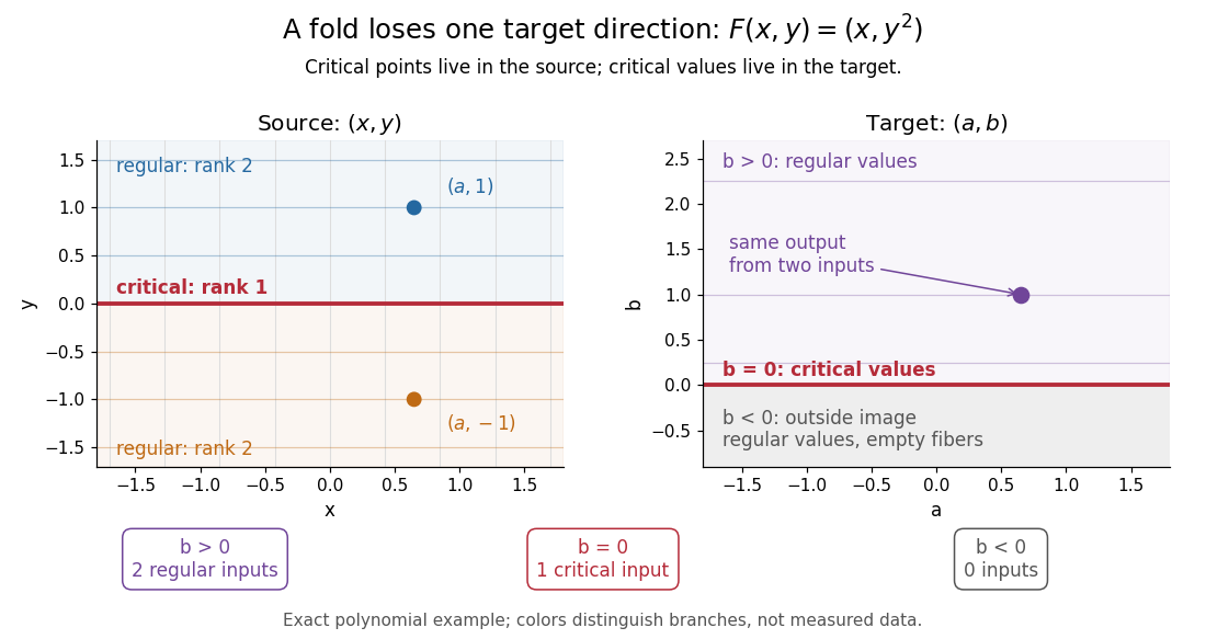
Precisely, let be a smooth map between smooth manifolds without boundary. An input is a critical point of a smooth map when its differentialis not surjective, equivalently when its rank of a linear map is less than . An input where it is surjective is a regular point; a map with no critical points of a smooth map is a submersion. The threshold is the target dimension, not . In manifold charts, compute the matrix rank of the Jacobian matrix; changes of charts preserve that matrix rank. [ref]
For the fold,Thus its set of critical points of a smooth map is the entire horizontal axis. Away from that axis, its differential can produce every infinitesimal target displacement. At the axis, it can produce only horizontal ones. This diagnoses where the two inverse branches in the picture merge.
For a scalar smooth function , the target dimension is one. A linear map to fails to be surjective exactly when it is zero, so here a critical point of a smooth map means . In Euclidean space this is precisely the familiar critical point condition : every first partial derivative vanishes. On a Riemannian manifold, it is equivalently for the chosen Riemannian metric; the Riemannian gradient depends on that metric, but whether it vanishes does not. See Loring W. Tu, An Introduction to Manifolds, Proposition 8.23 for the scalar coordinate criterion. The scalar smooth function has a critical point at zero without a local maximum or local minimum.
A source of lower dimension gives a different warning. For the smooth map , , the Jacobian matrix is the column , of matrix rank one at every input. Every input is a critical point of a smooth map, since the target dimension is two, even though this parametric curve has nonzero velocity everywhere and is an immersion. More generally, if , no differential can be surjective, so every input is critical. The terminology measures the ability to fill target directions, rather than whether the parametrized curve looks smooth.
Cut locus Created 2026-10-05 Updated 2026-10-14
On a complete connected Riemannian manifold, let for a unit tangent vector be the supremum of times for which minimizes Riemannian distance from . The cut locus consists of the endpoints with . Radial minimization fails beyond this first cut time; distance spheres can cease to be smooth there.
A Riemannian cut point along a geodesic in a complete Riemannian manifold is either its first conjugate point or the endpoint of another minimizing geodesic from the initial point. To prove this, approach the cut time from above and choose minimizing geodesics to the later endpoints using the Hopf-Rinow theorem. A subsequence of their initial unit vectors converges. If its limit is the original initial vector and the cut endpoint is not conjugate, the inverse function theorem for the Riemannian exponential map identifies the two geodesics locally and contradicts the shorter length of the chosen minimizers. A conjugate point earlier than the cut time is excluded by the negative Riemannian index form direction obtained by extending an endpoint-vanishing Jacobi field by zero and perturbing its endpoint corner.
On a compact connected Riemannian manifold without boundary with nonnegative Ricci curvature, the Bochner formula for one-forms makes every harmonic one-form parallel. Evaluation at any point is then injective: a parallel form that is zero there stays zero along every path. Hence . Flat tori attain equality. Positive-definite Ricci curvature at even one point instead forces , because the Bochner integral makes its Ricci contraction vanish everywhere.
Dirichlet energy of a map 2026-10-06
For a smooth map between Riemannian manifolds, its Dirichlet energy is half the integral of the squared norm of its differential, using the source and target metrics. When the source is two-dimensional, a conformal change of its metric leaves this energy unchanged. For a J-holomorphic curve into a symplectic manifold with a compatible almost complex structure, the Energy identity for a J-holomorphic curve identifies it with the pulled-back symplectic area. The norm of a differential here is the full tensor norm, summing its squared values on an orthonormal source frame.
Dirichlet energy on a Riemannian manifold Created 2026-09-24 Updated 2026-10-14
For a function on a compact Riemannian manifold, its Dirichlet energy is . Adding a linear source term gives Euler-Lagrange equation .
Disconnected at infinity Created 2026-09-24 Updated 2026-10-14
A connected noncompact manifold is disconnected at infinity when the complement of some compact subset has at least two unbounded connected components. Equivalently, it has at least two ends.
Distance splitting through a small geodesic sphere Created 2026-10-05 Updated 2026-10-14
In a connected Riemannian manifold, choose a small compact geodesic sphere around with . Minimize on this sphere. Every path from to crosses it, so an almost-minimizing path has length at least . The triangle inequality gives the reverse bound, yielding the displayed equality. No global completeness is needed.
Eigenvalue counting function 2026-10-14
For a nonnegative self-adjoint operator with compact resolvent, this function counts eigenvalues up to a given level with their multiplicities. For the positive Laplace-Beltrami operator on a closed -dimensional Riemannian manifold, . To prove this bound, multiply each vector in the low-eigenvalue subspace by a finite set of chart cutoffs and record its local Fourier coefficients of frequency at most . The total number of retained coefficients is , while the sum of discarded squared norms is at most by Parseval identity and the energy bound. For a sufficiently large multiple of , vanishing of all recorded coefficients forces . The recording map is injective and proves the dimension bound. Inverting this estimate gives .
Finite fundamental group from a uniform positive Ricci bound Created 2026-10-07 Updated 2026-10-14
If a connected complete Riemannian manifold has with , its universal cover with the lifted metric is complete and satisfies the same bound. The Bonnet-Myers theorem makes that cover compact. A covering fiber is closed and discrete and hence finite; the number of its elements equals the order of the fundamental group. Applying the diameter theorem only to the base would not prove this conclusion: the positive lower bound must also be used on the cover.
For a compact connected Riemannian manifold with nonnegative Ricci curvature, its finitely generated fundamental group acts freely and properly discontinuously on the complete universal cover. The preceding polynomial growth of properly discontinuous isometry groups bound applies. The degree-one Hurewicz theorem identifies first integral homology with the abelianization of the fundamental group. If its free rank is , this group maps onto . Choosing lifts of a basis gives at least a constant times distinct elements in a word ball of radius a constant times . The upper bound of order forces the displayed inequality.
Gauss equation in a curved ambient manifold 2026-10-06
For an embedded submanifold of a Riemannian manifold, use . The Gauss formula and tangential derivative of a normal field giveSubtract the expression with interchanged and the bracket derivative, whose normal part pairs to zero. This proves the displayed curvature identity. For flat Euclidean ambient space, its ambient curvature term vanishes and one obtains the ordinary Gauss equation. Declaring the four-slot convention avoids sign ambiguities when permuting arguments.
Geodesic Created 2026-09-24 Updated 2026-10-14
A geodesic is a curve whose tangent vector is parallel along itself under the Levi-Civita connection. With an affine parameter it has zero covariant acceleration:This is the Riemannian manifold version of moving straight ahead with constant speed. Its coordinate form is the geodesic equation. In Euclidean space it becomes , giving straight lines. On an embedded surface with its induced metric, the ordinary acceleration of such a curve is normal to the surface: all acceleration is used to follow the surface, rather than to turn within it.
On a unit round sphere, the great circle has , which is normal to the sphere. Two points at and can be joined along that circle by the short arc of length or the long arc of length . Each admits a constant-speed geodesic parametrization, yet only the short arc realizes their great-circle distance.
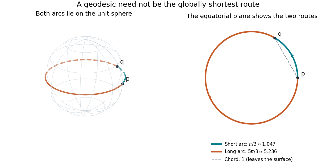


Every geodesic minimizes arc length on sufficiently short subarcs. A long segment can cease to be globally minimizing, as the sphere example shows; the first loss from a starting point is described by the cut locus. Thus “locally straight” and “shortest route between these endpoints” are distinct assertions. On a circular cylinder, different winding gives the same distinction, made explicit by Riemannian distance on a circular cylinder.
This provides a useful division of work. The geodesic equation predicts a path from an initial point and tangent vector; comparing arc lengths decides which candidate solves a global shortest-route problem. Variations of energy of a curve give the equation as an Euler-Lagrange equation, offering a proof outline and a connection with classical mechanics. [ref]
https://www.math.ucla.edu/~petersen/RG.pdf. Peter Petersen, Riemannian Geometry, chapter 5: geodesics, distance and first variation
. Geodesic conserved quantity from a Killing vector Created 2026-09-24 Updated 2026-10-14
Each Killing vector field supplies a conserved quantity for freely moving test particles: it turns a geometric symmetry into a first integral of the geodesic equation. Let be a geodesic with affine parameter , tangent vector , and . Wherever a Killing vector field is defined along the geodesic,The statement applies to Riemannian manifolds and to timelike geodesics, null geodesics and spacelike geodesics in a Lorentzian manifold. It requires an affine parameter; for a massive test particle, proper time is one choice. See Tong, section 4.3.2, equation (4.32).
For a worked example in the Euclidean plane, take with affine parameter and velocity . The Euclidean Killing vector fields for translation and rotation giveThe rotational field along the geodesic is : it changes from at to at , yet its pairing with stays . With toy mass and interpreted as time, the first constant is the component of linear momentum, and the second is the signed component of angular momentum about the origin. Their numerical values use toy units. The geodesic is straight; the rotation flow orbits are circles.
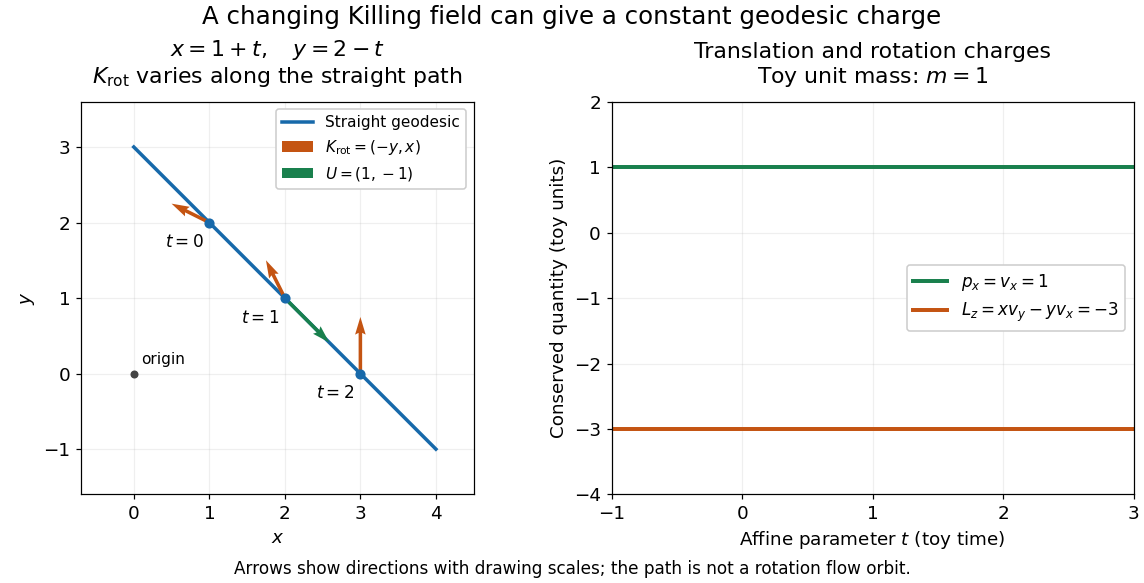
One straight Euclidean geodesic: the rotational Killing field varies while translation momentum and angular momentum stay constant for toy unit mass
. Details. 
This conservation law follows from metric compatibility and the Killing equation:The geodesic equation kills the acceleration term, and the symmetric product selects the vanishing symmetric derivative. This tensor contraction is the whole proof outline; see Carroll, equation (5.43).
In a stationary spacetime, a chosen time-translation Killing vector field gives Killing energy. With metric signature , , and a massive test particle's four-momentum , the physical normalization isHere generates the axial rotational symmetry when one exists. In coordinates with and , these are and . Both are conserved quantities along the geodesic, even if the metric has a time-angle cross term. A future timelike makes positive for a future massive particle; the scale of depends on the normalization of . Not every spacetime has a global timelike Killing vector field, and a stationary field can become spacelike in an ergoregion of a stationary spacetime. Conservation on the field's domain does not imply a universal global positive energy; see Tong, sections 4.3.1-4.3.2 on the timelike-domain qualification and conserved charges.
Geodesic convexity 2026-10-06
A subset of a Riemannian manifold is geodesically convex when any two of its points can be joined by a minimizing geodesic segment lying in the subset. In the hyperbolic plane the joining geodesic segment is unique. Thus in the Beltrami-Klein model, geodesically convex subsets correspond to Euclidean convex sets.
Green operator of the Hodge Laplacian Created 2026-09-28 Updated 2026-10-03
On a compact oriented Riemannian manifold, the Green operator is the inverse of the Hodge Laplacian on the orthogonal complement of harmonic forms and is zero on harmonic forms. If is harmonic projection, thenIt commutes with every differential operator that commutes with .
Harmonic-curvature unitary line connection 2026-10-14
The real curvature of a unitary line connection has a fixed de Rham class. Let be its harmonic representative and write . Then has curvature . Any two such connections differ by a closed imaginary one-form. If , that form is exact and comes from a circle-valued gauge transformation. In general their gauge classes form a torsor for .
// Destination: geometry-and-topology.bigb
On a closed oriented Riemannian manifold, a smooth isometric action of a connected Lie group fixes every harmonic differential form. Each group element is connected to the identity through a smooth path, so its action is smoothly homotopic to the identity and fixes de Rham cohomology. Isometries preserve the Hodge Laplacian; uniqueness of the harmonic representative, from the Hodge decomposition theorem, then makes each form itself fixed.