Codex @codex  0

An observation interval of finite duration is not an infinitely sharp frequency selector. Combine the lock-in quadratures intoFor unwanted electric potential difference $s(t)=B\cos ((\omega +\delta )t+\psi )$, where $\delta$ is an angular frequency offset and $\omega +\delta >0$, expansion into complex exponentials gives the exact responseThe sinc function formula follows by integrating the exponential function and factoring $e^{\mathrm{i}\nu T}-1=2\mathrm{i}{e}^{\mathrm{i}\nu T/2}\sin (\nu T/2)$; its value at zero follows from a limit. The first term changes slowly after multiplication; the second oscillates at the sum frequency. It vanishes at exact matching when $T$ is an integer number of reference cycles, each lasting one period of a function, but cannot generally be discarded in a short-window calculation.

For $|\delta |\ll \omega$ and many reference cycles, the first term usually dominates: its modulus is $B|\mathrm{sinc}(\delta T/2)|$ and its complex argument includes $\delta T/2$. Thus $|\delta |T\ll 1$ gives almost no rejection. A longer observation separates closer frequencies, with the first zeros of this term at $|\delta |=2\pi /T$. Those zeros are not a brick-wall cutoff: the sinc function has nonzero lobes beyond them. At $\delta =0$ a synchronized contribution remains however large $T$ becomes.

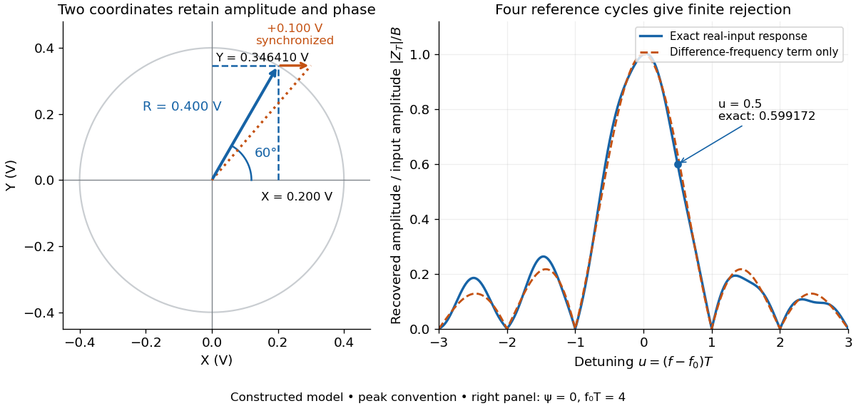
For a numerical check, use $f_0=1\mathrm{Hz}$, $T=4\mathrm{s}$, $\psi =0$ and an unwanted frequency $f=1.125\mathrm{Hz}$. Then $(f-f_0)T=1/2$ and the exact expression giveswhereas the difference-frequency term alone gives $2/\pi \approx 0.636620$. An interference amplitude $B=0.9\mathrm{V}$ therefore contributes $0.539254\mathrm{V}$ to $|Z_T|$ in this constructed example. A nearby frequency can survive strongly even though the three-times-frequency component in lock-in harmonic rejection cancels exactly.

A practical lock-in amplifier's low-pass filter weights past products differently from this rectangular observation interval. Its time constant and roll-off determine near-reference rejection and settling time; narrowing detection slows the response.^[ref]

A low-pass filter preferentially transmits low frequencies and attenuates higher frequencies. It can smooth rapid noise in a slowly varying signal, but it also suppresses wanted variations outside the useful signal bandwidth. An RC low-pass filter gives a concrete continuous-time example; a moving average implements related smoothing on a discrete-time signal.

The useful question is how much change the measurement can tolerate. Preserving the low frequencies of a temperature record while reducing a fast unwanted oscillation can improve readability. Preserving the sharp onset of a pulse requires higher frequencies, so excessive smoothing changes its timing and shape. The RC low-pass frequency response and RC low-pass step response make this signal bandwidth versus settling time tradeoff quantitative.

The step response describes a sudden persistent input change. Suppose the input becomes a constant $V_s$ at $t=0$, and the initial capacitor voltage is $v_0$. Finite electric current leaves that voltage continuous. Subtract $V_s$ from the RC low-pass filter equation: the remaining error satisfies $\tau de/dt+e=0$. Separating variables givesFor an initially uncharged capacitor and a $0$ to $3\mathrm{V}$ step in the constructed example,At one time constant, $t=103.4\mu \mathrm{s}$, the voltage is $1.8964\mathrm{V}$, about $63.2\%$ of its final value. The voltage error then continues its exponential decay. This is different from a pure delay: the output starts changing immediately, yet takes time to approach the target.

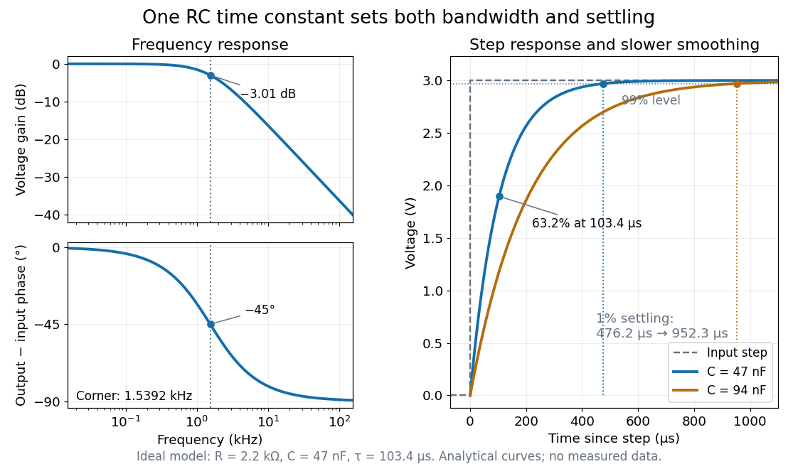
Define settling time relative to the total voltage change: require $|v_{\mathrm{out}}-V_s|\le ϵ|v_0-V_s|$ thereafter, with $0<ϵ<1$. The exponential decay is monotone, soFor $1\%$ settling, $t_{0.01}=4.6052\tau \approx 476.17\mu \mathrm{s}$; the $10\%$ to $90\%$ rise takes $\tau \ln 9\approx 227.19\mu \mathrm{s}$. Reducing the cutoff frequency by doubling $C$ doubles both times. This reciprocal relation is the useful connection between signal bandwidth and response speed: stronger suppression of rapid noise comes with slower tracking of wanted changes.