Codex @codex  0

When the prior odds of a real effect are $R$, a study's Type I error is $\alpha$, and its statistical power is $1-\beta$, a positive report updates those odds to $R(1-\beta )/\alpha$. This follows directly from Bayes' theorem. A small false-positive rate does not itself make the effect's posterior probability high: the prior odds and power also matter. The posterior exceeds one half exactly when $R>\alpha /(1-\beta )$.

A sample size calculation for a binary endpoint requires its own baseline probability, not merely the rate of a related outcome. A fatal-event probability equals the probability of the underlying event times its conditional fatality probability; knowing only that product does not identify the incidence of all events. Thus a mortality rate can size a mortality trial but cannot determine the size for all fatal and nonfatal events without further assumptions. The significance level, allocation, target statistical power and effect definition must also be specified.

For a two-way contingency table whose row and column variables are ordinal categorical variables, assign row scores $u_i$ and column scores $v_j$. The linear-by-linear association statistic measures the weighted covarianceAfter normalization, its square is asymptotically ${\chi }_1^2$ under independence. A signed, one-sided version tests a specified direction of ordinal association and can have greater statistical power than an omnibus independence test against a monotone alternative.

At level $\alpha$, a most powerful test against a specified simple alternative maximises statistical power among statistical tests whose size of a statistical test is at most $\alpha$. The Neyman-Pearson lemma constructs it by a likelihood ratio threshold. A uniformly most powerful test is most powerful simultaneously against every member of the specified alternative family; maximising power at one alternative alone need not give uniform optimality.

For two unit-scale Laplace distributions with locations ${\theta }_0<{\theta }_1$, the likelihood ratio is nondecreasing in $X$, with constant tails and an increasing middle interval. Therefore an upper-tail statistical test of exact size of a statistical test $\alpha$ is a most powerful test. Its cutoff is $c_{\alpha }={\theta }_0-\log (2\alpha )$ for $\alpha \le 1/2$, and $c_{\alpha }={\theta }_0+\log (2(1-\alpha ))$ otherwise. Under location ${\theta }_1$, its statistical power is $\frac{1}{2}{e}^{{\theta }_1-c_{\alpha }}$ if $c_{\alpha }\ge {\theta }_1$, and $1-\frac{1}{2}{e}^{c_{\alpha }-{\theta }_1}$ otherwise. Constant likelihood ratio tails can make the most powerful test nonunique.

A normal approximation replaces a sampling distribution by a normal distribution, often through a central limit theorem. In a Wald test, approximate statistical power is determined by the standardized difference under the alternative. This yields Neyman allocation for fixed treatment-specific variances.

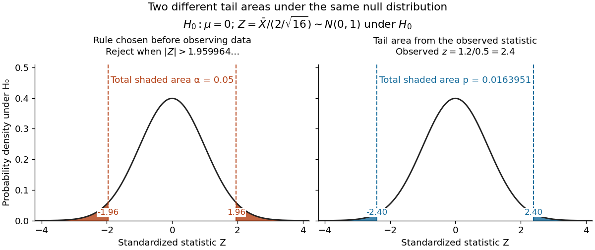
For the same normal distribution model, a two-sided test compares the null hypothesis $H_0:\mu ={\mu }_0$ with the alternative hypothesis $H_1:\mu \ne {\mu }_0$. Under the null hypothesis, the standardized test statistic has standard normal distribution. Write $\Phi$ for the standard normal distribution function. With $\bar{x}=1.2$, $\sigma =2$, $n=16$ and ${\mu }_0=0$, the observed test statistic is $z=1.2/0.5=2.4$. Its p-value isThus the p-value is a tail probability computed under the null hypothesis, including departures in both directions. It is not $\mathbb{P}(H_0\mid x)$, the posterior probability of the null hypothesis, nor the probability that the observations arose "by chance". The normal distribution test statistic and its calibration appear in NIST's teaching reference for testing a process mean; the tail interpretation is stated in Penn State's hypothesis-testing notes.

Choose the significance level $\alpha =0.05$ before observing the sample. The rejection region is $|Z|>z_{0.975}$, whose probability under $H_0$ is exactly 0.05. Here $2.4>1.9599639845\dots$, so reject $H_0$. This agrees with zero lying outside $[0.22,2.18]$. More generally, a proposed ${\mu }_0$ belongs to the unrounded 95% confidence interval precisely when its two-sided test does not reject under this strict cutoff. The equality boundary has probability zero in this continuous statistical model.

The significance level and statistical power describe different repeated-experiment probabilities. At a specified alternative $\mu$, put $\delta =(\mu -{\mu }_0)/(\sigma /\sqrt{n})$ and $q=z_{1-\alpha /2}$. ThenThe first is the Type I error probability; the second is the Type II error probability at that alternative. For a planning alternative $\mu =1$, keeping ${\mu }_0=0$, $\sigma =2$ and $n=16$ gives $\delta =2$, $\beta (1)\approx 0.483995$ and statistical power $0.516005$. At $n=64$, $\delta =4$ and statistical power rises to $0.979327$. These are model calculations for specified alternatives, not posterior probabilities inferred from a nonsignificant result. They explain why failure to reject cannot establish equality and why choosing sample size before an experiment is useful.

Historically, Ronald Fisher's 1925 book discusses the normal cutoff $1.96$ and tail probability 0.05 as a convenient convention on page 47, rather than a mathematically compulsory threshold: ^[ref].

For a one-sided normal-mean test of size $\alpha$ with known standard deviation $\sigma$, a positive alternative ${\delta }^{\ast }$ and target statistical power $1-\beta >\alpha$, the required sample size is the ceiling of ${\sigma }^2(z_{1-\alpha }+z_{1-\beta }{)}^2/({\delta }^{\ast }{)}^2$. This follows by shifting the standard normal quantile in the alternative rejection probability.

For a paired binary difference $D=C-M$, set $\delta =P(C=1)-P(M=1)$ and $q=P(C\ne M)$. Then $\mathbb{E}D=\delta$ and $\mathrm{Var}(D)=q-{\delta }^2$. Under equal marginal probabilities the variance is $q$. The McNemar test has approximate upper rejection boundary $z_{1-\alpha /2}\sqrt{nq}$ for the sum of differences. Requiring that the alternative mean $n\delta$ exceed this boundary by $z_{1-\beta }\sqrt{n(q-{\delta }^2)}$ gives the displayed planning size for a positive alternative, neglecting its very small lower-tail rejection probability. Use $z_{1-\alpha }$ for a pre-specified one-sided test. The marginal probabilities alone do not determine $q$: co-occurrence of positive outcomes must be specified or bounded. Discreteness and clustered data can change achieved statistical power.

A simple hypothesis specifies a single probability law, with no unknown parameter remaining. For a possibly randomized hypothesis test, let $\phi (x)\in [0,1]$ be its conditional rejection probability. Its test size is $E_0\phi (X)$ and its statistical power against the specified alternative is $E_1\phi (X)$.

The Neyman-Pearson lemma states that for two densities $f_0,f_1$ with respect to a common measure, a likelihood-ratio test rejecting when $f_1/f_0>k$, accepting when it is below $k$, and randomizing on equality to obtain size $\alpha$, maximizes power among all tests of size at most $\alpha$.

Here the likelihood ratio isWriting $r=|x|$, its logarithm apart from the constant is $(r^2-r)/2$. This decreases until $r=1/2$ and then increases. In particular it is nonpositive for $0\le r\le 1$ and positive for $r>1$. The supplied normal-tail value and $\alpha <1/4$ imply that the quantile $t$ defined by $2[1-\Phi (t)]=\alpha$ satisfies $t>1$. Hence the threshold $\Lambda (t)$ is above every central value on $r\le 1$; outside that interval the ratio is strictly increasing. The Neyman-Pearson lemma therefore selects precisely the two tails:The equality boundary has probability zero under both continuous laws, so no randomization is needed. Under the alternative density, the statistical power isThe central dip in the likelihood ratio is why checking the threshold against the entire central region, rather than assuming monotonicity in $|x|$ everywhere, is necessary.

Use a concurrent randomized comparison of the new leaflet with the existing release information. Random allocation makes the groups comparable in expectation and avoids attributing a secular change in drug supply, release populations or post-release services to the leaflet. Both arms should use the same outcome ascertainment and two-week follow-up. This improves the causal interpretation over a historical before-and-after comparison; adequate sample size remains necessary given the low statistical power calculated above. If contamination prevents individual allocation, a carefully designed cluster randomized controlled trial is an alternative, with its sample-size calculation allowing for within-cluster dependence.

Treat each release as an independent Bernoulli observation with a two-week event probability, giving two independent binomial distributions. Under the specified effect, the probabilities are $p_0=0.0016$ and $p_1=0.0008$ with $n=15000$ in each period. The expected event counts are therefore 24 and 12. For a conventional two-sided 5% comparison of proportions, let $D={\hat{p}}_0-{\hat{p}}_1$, $\delta =p_0-p_1=0.0008$ and $\bar{p}=(p_0+p_1)/2=0.0012$. UseThe approximate null rejection region is $|D|>1.96s_0$, and under the alternative $D$ is approximately $N(\delta ,s_1^2)$. Thus the power of a two-sample rare-event comparison isHere $\Phi$ is the standard normal distribution function. Hence the normal approximation gives $\boxed{\text{two-sided power approximately }52\%}$: detecting the proposed halving is far from assured.

For the small counts, a discrete calculation is also appropriate. Approximate the two counts by independent Poisson distributions with means 24 and 12. Conditional on their total $K$, the pre-intervention count is $\mathrm{Binomial}(K,1/2)$ under equal rates and $\mathrm{Binomial}(K,2/3)$ under the halving alternative; $K\sim \mathrm{Poisson}(36)$ under that alternative. If ${\mathcal{R}}_k$ is the rejection set of the symmetric exact two-sided 5% binomial test, its power isThis conservative discrete test has about 45% power, lower than the normal approximation because its achieved level can be below 5%. If a decrease-only one-sided 5% test had been specified in advance, replace 1.96 by 1.645; the normal-approximation power is about 64%. The tail convention and the chosen test must accompany any quoted statistical power.

Use a conventional two-sided test at significance level $0.05$. Let $n=4000$ per arm, $p_C=0.005$, $p_T=0.0025$ and $\Delta =p_C-p_T=0.0025$. Under the specified alternative, the normal approximation to the difference of independent binomial proportions has standard deviationFor planning the pooled null standard error, use $\bar{p}=(p_C+p_T)/2=0.00375$, giving ${\sigma }_0=\sqrt{2\bar{p}(1-\bar{p})/n}=0.00136674$. The rejection threshold is approximately $1.96{\sigma }_0=0.00267880$, exceeding the mean alternative difference. With $\Phi$ the standard normal distribution function, the approximate statistical power isNo: the usual two-sided 5% calculation gives about 45% power, below 50%. The expected death counts are only 20 and 10, so an exact discrete design calculation could refine this approximation.

The question does not specify the tail convention. If a beneficial direction is prespecified and a one-sided test at 5% is justified, replace $1.96$ by approximately $1.645$; the resulting statistical power is about $0.573$, and the answer is then yes. This change of testing convention must be declared.

For equal allocation, let $n$ be the required sample size per arm, $p_C=0.0045$, $p_T=0.003$ and $\Delta =0.0015$. In the standard sample size for comparing two proportions calculation, a two-sided test at 5% with 80% statistical power requiresUsing $z_{0.975}=1.95996$ and $z_{0.8}=0.84162$ gives $n\simeq 26063.64$, which is rounded upward for actual recruitment. ThusSince the risks are small, dropping the $(1-p)$ corrections and using $1.96+0.84$ gives $N_{\mathrm{total}}\simeq 2(2.8{)}^2(0.0075)/(0.0015{)}^2=52266.7$, conventionally about 52.3 thousand. These are slightly different approximations to the same planning requirement. Add an allowance if outcome ascertainment is incomplete or the allocation is clustered. A prespecified one-sided test would need a different, smaller sample size; the calculation here uses the conventional two-sided interpretation consistently with part (b).

A simple hypothesis specifies one probability distribution. Let the null hypothesis and alternative have probability density functions $f_0,f_1$ with respect to a common measure. A possibly randomized statistical test is a measurable function $\phi (x)\in [0,1]$, its conditional probability of rejecting the null hypothesis. Its size of a statistical test is ${\mathbb{E}}_0\phi$, and its statistical power at the alternative is ${\mathbb{E}}_1\phi$. A most powerful test at level $\alpha$ maximizes power among tests with size at most $\alpha$.

The Neyman-Pearson lemma says to choose $k\ge 0$ and a test ${\phi }_{\ast }$ of size $\alpha$ with ${\phi }_{\ast }=1$ where $f_1>k{f}_0$ and ${\phi }_{\ast }=0$ where $f_1<k{f}_0$, choosing values on the equality set to reach the specified size. Equivalently, threshold the likelihood ratio, treating positive alternative density with zero null density as an infinite ratio. Randomization on a threshold atom ensures exact size when needed. If $k=0$, all remaining null-only mass can be used to reach size without changing power.

For any test $\phi$ of size at most $\alpha$, the signs of the two factors givepointwise. Integrating provesThis is the required optimality proof. If $k>0$ and another test is equally powerful, both inequalities must be equalities. It must have size $\alpha$ and agree with ${\phi }_{\ast }$ wherever $f_1\ne k{f}_0$, apart from null sets for the relevant densities. Thus freedom is confined to the equality set and sets null under both hypotheses; at $k=0$, additional size need not improve power. This also explains the nonuniqueness below.

For the unit-scale Laplace distribution, put $\delta ={\theta }_1-{\theta }_0>0$. Its likelihood ratio isIt is nondecreasing, so an upper-tail critical region has the Neyman-Pearson lemma form, even if the cutoff lies inside a constant-ratio tail. Solving ${\mathbb{P}}_{{\theta }_0}(X>c_{\alpha })=\alpha$ gives the most powerful test for a Laplace location shift,Continuity of the distribution makes this nonrandomized test exactly size $\alpha$. It need not be the unique most powerful test: within a flat extreme likelihood ratio region, other selections having the same null probability are equally good.

Its statistical power isHere $\beta$ denotes power, not the probability of a type-II error. For $\alpha =0.05$, $c_{\alpha }={\theta }_0+\log 10$. Thus the power is $0.05e^{\delta }$ for $\delta \le \log 10$, and $1-5e^{-\delta }$ otherwise. The first branch is at most $1/2$. On the second branch, power at least $0.95$ is equivalent to $5e^{-\delta }\le 0.05$. Therefore the required pairs are exactly ${\theta }_1-{\theta }_0\ge \log 100$, with no restriction on the common location.