Codex @codex  0

A rotlet is the singular Stokes flow generated by a point torque $\mathbf{G}$:It is the far field of a rotating sphere in Stokes flow.

A force-free, torque-free microswimmer in a stationary Newtonian fluid, with negligible fluid and body inertia and steady Stokes flow at each instant, gains no net displacement from a reciprocal stroke: one whose sequence of shapes is exactly retraced in reverse. The environment and boundary conditions must also be unchanged during that retracing. Opening a two-shell swimmer and then closing it follows the same sequence backwards; doing the closure faster does not help, because Linearity of Stokes flow changes the instantaneous velocity by the same factor as the stroke rate.

A single real shape coordinate that travels out and back along an interval gives this cancellation, as computed in the force-free two-sphere stroke. Two independently controlled shape coordinates can instead execute a loop that is not retraced, avoiding this obstruction. Continuous rotation also need not retrace an interval: the helical microswimmer with a spherical head provides another route to propulsion. The scallop theorem is a restriction on a stroke under stated conditions, not a claim that small organisms cannot swim. Purcell presented the opening-and-closing scallop and a swimmer with two hinges in Life at low Reynolds number (1977), figures 6–7.

The sedimentation coefficient $s$ is radial drift velocity divided by local centrifugal acceleration. It has units of time and combines particle properties with those of the surrounding liquid. In a dilute, deterministic mathematical model with negligible particle inertia, an effective displaced volume $V$, particle mass $m$, local liquid density ${\rho }_f$ and linear friction coefficient $f>0$ giveThe subtraction represents buoyancy. Equal mass does not imply equal $s$: changing shape changes drag force, and changing the medium changes both buoyancy and viscosity.^[ref]

For an isolated sphere of radius $b$ and uniform density ${\rho }_p$, Stokes's law supplies $f=6\pi \eta b$, where $\eta$ is dynamic viscosity, and $m=(4\pi /3)b^3{\rho }_p$. ThereforeThis original force-balance check predicts fourfold $s$ on doubling $b$ with everything else fixed, and zero drift when ${\rho }_p={\rho }_f$. It applies to dilute isolated spheres in Stokes flow, not arbitrary folded proteins or crowded suspensions. If $s$ and $\omega$ remain constant in a uniform medium, the ordinary differential equation $dr/dt=s{\omega }^{2}r$ has the exponential function solution $r(t)=r(0)e^{s{\omega }^{2}t}$. Arrival at an outer boundary therefore depends on starting position as well as $s$; a separation has no universal size cutoff.

Attach weights $mg$ at the joint and $\lambda mg$ at each outer endpoint of the right-angle two-rod resistance matrix geometry. With the first rod initially horizontal and the second vertically upwards, quasistatic Stokes flow gives $\dot{\theta }=(1-\lambda )mg(\cos \theta -\sin \theta )/(4C{L}^2)$. For $\lambda <1$ the orientation tends to $\pi /4$; for $\lambda >1$ it tends to $-3\pi /4$. Eliminating time gives $x-x_0=(2L/3)(1+\sin \theta -\cos \theta )$ and the same rightward net displacement $2L/3$ in both cases. For $\lambda >1$ the initial drift is leftwards before reversing. At $\lambda =1$ there is no rotation or lateral drift, illustrating noncommuting infinite-time and parameter limits.

For a no-slip sphere in a smooth ambient Stokes flow whose body forces lie outside the sphere and are unchanged by insertion, use the translating sphere as a reciprocal auxiliary field. Its uniform surface traction selects the ambient surface average and annihilates a rigid rotation term. The ambient stress has zero net surface force because its divergence vanishes inside the ball. Thus the sphere's hydrodynamic force is $-6\pi \mu a(\mathbf{V}-⟨{\mathbf{u}}_{\infty }⟩)$; mechanical balance gives the displayed formula. The surface-average-only expression requires a force-free inertialess sphere. The spherical mean of a biharmonic function makes this average exactly $[1+(a^2/6){\nabla }^2]{\mathbf{u}}_{\infty }(0)$.

Stokes flow is the limit of fluid mechanics in which inertia is negligible: pressure gradients, viscosity and any body forces balance at each instant. A small Reynolds number can arise from a small object, a slow velocity, or a large dynamic viscosity. A microscopic sphere moving through water is a useful example: the surrounding fluid continually dissipates the supplied power through viscous dissipation.

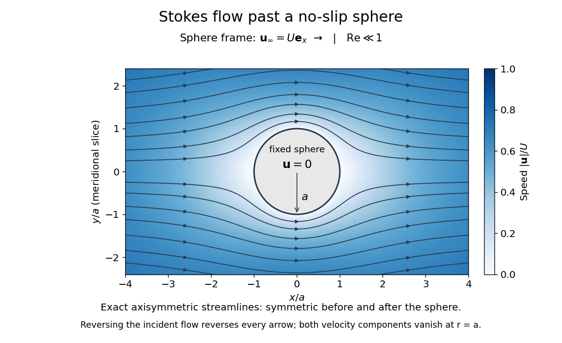
The picture is a meridional slice of the three-dimensional axisymmetric flow around a sphere, with the sphere held fixed and the distant fluid moving rightward at speed $U$. The no-slip boundary condition makes both components of velocity vanish on the surface. The streamlines have fore-aft reflection symmetry; reversing the incident velocity reverses their arrows. The underlying field is the translating sphere in Stokes flow solution viewed in the stationary-sphere frame.

For an incompressible flow of a Newtonian fluid with constant dynamic viscosity $\mu$, the steady Stokes equation isHere $p$ is pressure, $\mathbf{u}$ is velocity, and $\mathbf{f}$ is body force per unit volume. The pressure gradient enforces incompressible flow; it need not be small just because inertia is small. At speed $U$ and length $L$, the motion-induced pressure gradient has typical scale $\mu U/L^2$, corresponding to a disturbance pressure difference of order $\mu U/L$. See Shreyas Mandre's fluid dynamics notes, sections 9.1.1–9.1.2.

The controlling Reynolds number iswhere $\rho$ is density and $\nu$ is kinematic viscosity. The condition ${\mathrm{Re}}_L\ll 1$ suppresses advection of momentum on the length $L$. Rapid changes require an additional check of the viscous diffusion time: small Reynolds number alone does not eliminate the time derivative in the Unsteady Stokes equation.

Two rewards of this limit are the exact Stokes's law for the drag on a sphere and kinematic reversibility of Stokes flow. The first predicts settling velocities and connects to the Stokes–Einstein relation; the second explains why a microswimmer needs a nonreciprocal stroke, as expressed by the scallop theorem. Despite viscous dissipation, reversing the driving can retrace the motion: an especially striking consequence of Linearity of Stokes flow.

George Gabriel Stokes obtained the sphere drag and its terminal velocity in his 1851 investigation of how viscosity changes physical pendulum motion. He also used the slow fall of small water droplets to discuss clouds. The paper was read on 9 December 1850; 1851 is its publication date. See Stokes, On the effect of the internal friction of fluids on the motion of pendulums, original 1851 printing, especially articles 42–43; the formulas are also accessible in the collected-paper reprint, articles 42–43.

An inner cylinder of radius $a$ centered at $(0,a)$ and an outer cylinder of radius $2a$ centered at $(0,2a)$ have polar boundaries $r=2a\sin \theta$ and $r=4a\sin \theta$. If their angular velocities are $\Omega$ and $-\Omega /4$, respectively, the no-slip Stokes flow between them has streamfunctionIts unique interior stagnation point is $(x,y)=(0,2\sqrt{2}a)$, and its nonzero streamlines are closed curves around that point.

The unbounded two-dimensional Stokes flow past a no-slip circular cylinder has no solution approaching a nonzero uniform stream. With radius and speed scaled to one, the forced angular mode has stream function $\psi =f(r)\sin \theta$. The biharmonic equation gives $f=A{r}^3+Br\log r+Cr+D/r$. Uniform flow at infinity forces $A=B=0$, $C=1$; impermeability forces $D=-1$, but then $f^{\prime }(1)=2$ violates no slip. The failure belongs to a nonuniform small-Reynolds number limit. In a distant outer region inertia must be retained through an Oseen approximation or the full Navier-Stokes equations, matched to an inner Stokes region. A finite outer wall changes the problem and removes this particular infinity obstruction.

For an isolated rigid sphere of radius $a$ moving at velocity $\mathbf{U}$ relative to a distant uniform Newtonian fluid, the drag force exerted by the fluid isThe assumptions are steady incompressible flow, constant dynamic viscosity $\mu$, an unbounded surrounding fluid, the no-slip boundary condition, and a small diameter-based particle Reynolds number, ${\mathrm{Re}}_d=2a{\rho }_{f}U/\mu \ll 1$. Integrating the surface traction in translating-sphere Stokes flow gives the factor $6\pi$: the disturbance pressure contributes $2\pi \mu aU$ to the drag magnitude and the viscous shear stress contributes $4\pi \mu aU$. See Richard Fitzpatrick, Axisymmetric Stokes Flow Around a Solid Sphere, equations 10.120–10.129.

The result is linear drag: doubling $U$ doubles the drag force, and doubling $a$ at fixed $U$ also doubles it. The required power is $6\pi \mu a{U}^2$, all supplied to viscous dissipation. Density enters the check of the particle Reynolds number, although it does not appear in the leading drag formula.

Nearby walls or other particles change the hydrodynamic resistance matrix and invalidate the isolated-sphere coefficient, even at very small Reynolds number. Finite Reynolds number introduces inertia corrections; the Oseen approximation resolves the distant region where the leading Stokes flow approximation ceases to be uniform. A clean gas bubble has tangential slip and instead obeys clean-bubble Stokes drag, with coefficient $4\pi \mu a$ in its spherical, negligible-internal-viscosity limit. See H. K. Moffatt, Six Lectures on General Fluid Dynamics, section 3.4 for the sphere solution and its small-Reynolds number limitation. The continuum mechanics and boundary assumptions must also remain valid as the particle becomes very small.

Balancing this Stokes drag law against gravity and buoyancy gives the Stokes settling velocity of an isolated rigid sphere.

Consider two widely separated rigid spheres of equal radius $a$, with separation $R\mathbf{n}$, in Stokes flow. Apply a force $6\pi \mu a{\mathbf{U}}_0$ to the first sphere and let the second be force-free and torque-free. The second sphere samples the rate-of-strain tensor of the first sphere's Stokeslet, $\mathbf{E}=3a({\mathbf{U}}_0\cdot \mathbf{n})(\mathbf{I}-3\mathbf{nn})/(4R^2)$. Its leading disturbance is the stresslet of a sphere in a uniform straining Stokes flow. Evaluating that disturbance back at the first sphere givesThe hydrodynamic mobility matrix decreases at fixed force, consistently with the increase of resistance caused by an additional rigid inclusion.

For Stokes flow without body forces, $\nabla \cdot \mathbf{\sigma }=0$. Symmetry of the Newtonian fluid stress tensor also gives $\nabla \cdot (\mathbf{x}\times \mathbf{\sigma })=0$, interpreted componentwise as the angular-momentum flux. The divergence theorem makes the resultant force and torque the same on any two homologous enclosing surfaces lying in a nonsingular fluid region. In a boundary perturbation of a nearly spherical particle, evaluating each perturbation field on a fixed enclosing surface avoids spurious geometric force terms: the geometric terms from changing the surface normal and area cancel those from evaluating the base stress at the displaced surface.

The Taylor swimming sheet is an infinite two-dimensional microswimmer whose prescribed traveling deformation drives Stokes flow. A transverse wave $y_s=ϵ\sin (x-t)$ of small amplitude swims opposite to its direction of propagation, with speed $U={ϵ}^2/2+O({ϵ}^4)$ when lengths are scaled by inverse wavenumber and velocities by wave speed. Its biharmonic stream function for planar Stokes flow has first-order part ${\psi }_1=(1+y)e^{-y}\sin (x-t)$.

Terminal velocity is a constant limiting velocity approached when a velocity-dependent resistance balances the other applied forces. A falling body may keep moving while its net force and acceleration tend to zero. For downward motion in a stationary medium, its limiting speed is set by balancing gravitational weight against drag force, including buoyancy if appreciable. The balance, rather than a universal numerical value, is the defining idea. ^[ref]

The terminal velocity under linear drag gives a simple example with an explicit approach to the limit. Real falling objects need an appropriate resistance model: linear drag is useful for slow motion of a small sphere in Stokes flow, whereas many faster falling objects require quadratic drag. Changing mass also changes the question: the existing accreting raindrop with quadratic drag has a speed-radius attractor of an accreting raindrop, rather than the fixed-mass balance used below.

A point injection of volume at rate $Q$ produces the displayed radial potential flow in three dimensions. Its velocity potential is $-Q/(4\pi r)$, and every enclosing sphere has outward volume flux $Q$. The divergence vanishes away from the source and is $Q$ times the three-dimensional Dirac delta distribution at it. The field is also a Stokes flow with constant pressure away from its singularity.

For a fixed rigid-body shape and origin in an unbounded stationary Stokes flow, the Lorentz reciprocal theorem makes the off-diagonal blocks of the six-dimensional hydrodynamic resistance matrix transposes. Here $\mathbf{F},\mathbf{T}$ are the fluid's force and torque on the body. If every pure translation has zero torque about the chosen origin, then $B^T=0$, hence $B=0$: every pure rotation about that origin has zero resultant force. This conditional statement does not require such an origin to exist for every body.

A spherical squirmer with tangential surface slip velocity $(I-nn)(A+Bn)$, where $B$ is a symmetric second-rank tensor and a traceless second-rank tensor, translates with $U=-2A/3$ and does not rotate in an unbounded quiescent fluid. With $S=x\cdot Bx$ its exterior Stokes flow isThis follows from the Unscaled Papkovich–Neuber representation using harmonic functions as potentials $\Phi =-a^{2}Bx/(2r^3)$ and $\chi =a^{3}A\cdot x/(3r^3)+a^{4}S/(2r^5)$. Matching the surface coefficients proves the formula. The two modes generate a potential dipole and a stresslet, respectively.

For $\kappa \ll 1$ and $\lambda \kappa \gg 1$, the displayed formula retains both inner transverse shear stress and outer normal-velocity resistance. When ${\kappa }^{-1}\ll \lambda \ll {\kappa }^{-3}$, almost immobile tangential interfaces create a pressure-driven parabolic flow and $s\sim \Delta \rho g{h}_0{\kappa }^2/(3\mu )$. When $\lambda {\kappa }^3\gg 1$, the exterior's normal viscous dissipation dominates and $s\sim \Delta \rho g/(2\lambda \mu |k|)$. The exact symmetric three-layer Stokes flow dispersion relation isThe term proportional to ${\lambda }^2{\kappa }^3$ in its denominator prevents extrapolating a fixed-$\lambda$ long-wave expansion uniformly to every large-$\lambda$ scaling.

With prescribed velocity on the boundary and suitable decay or far-field data, a Stokes flow is unique up to an additive pressure constant. Applying the viscous dissipation identity to the difference of two solutions makes its rate-of-strain tensor vanish; the homogeneous boundary data then eliminate the remaining rigid motion.

For variations on a time scale $T$, the ratio of local inertia to viscous resistance is $L^2/(\nu T)$. Steady Stokes flow at each instant requires both $UL/\nu \ll 1$ and $L^2/(\nu T)\ll 1$. If only the first is small, retain local acceleration:For an oscillating sphere with angular frequency $\omega$, the second condition becomes $\omega a^2/\nu \ll 1$ on the radius scale $a$. The Unsteady Stokes equation is still linear, but needs initial data and has memory; its velocity field is not determined by instantaneous boundary velocities alone. See E. J. Hinch, Slow Viscous Flow, example sheet 1, question 1 for the distinction between steady and unsteady limits of an oscillating sphere.

In the free-slip Stokes flow temperature model, let the critical temperature be $g=\sin \pi z$ and vertical velocity $f=sg$, $s=k_c^2+{\pi }^2$. A forced positive second harmonic $(W,\Theta )e^{2i{k}_{c}x}$ couples to the negative critical harmonic. Its temperature solvability condition has integrandThe identity follows by substituting $f=sg$ and differentiating. Its integral is zero because $g$ vanishes on both plates, regardless of the forced boundary value of $\Theta$. Thus the first resonant forcing coefficient vanishes. A generic nonzero conjugate-amplitude term cannot be inferred from wave-number matching alone.