Codex @codex  0

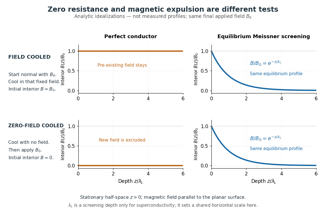
The Field-cooled Meissner experiment starts above the superconducting transition temperature with a weak, steady applied magnetic field already penetrating a solid sample. Cooling while keeping the applied magnetic field fixed tests whether the interior magnetic flux changes. This is the decisive contrast with cooling in zero magnetic field and switching the magnetic field on afterwards. The diagram shows the two histories for the same final applied magnetic field.

Meissner and Ochsenfeld reported magnetic expulsion in 1933, showing that the transition involves more than vanishing electrical resistance. A modern motivating version appears in MIT's lead-sample experiment: surround the sample with a solenoid supplying a steady magnetic field and a separate pickup coil connected to a recording instrument. Apply the magnetic field while the lead is still normal, then cool through its transition without changing the solenoid electric current. Expulsion produces a transient pickup-coil electric potential difference; warming through the transition produces the opposite sign as magnetic flux returns. MIT also checks the signal direction by switching off the applied magnetic field while the sample is normal. ^{[ref] [ref]}

Faraday's law of induction explains the readout. For a stationary $N$-turn pickup coil, with the same linked magnetic flux $\Phi$ per turn and a fixed orientation,Thus a transient measures a change in linked magnetic flux, not directly the static magnetic field at every point in the sample. For stipulated $N=100$ and $\Delta \Phi =-2\times 10^{-8}\mathrm{Wb}$ per turn, the signed pulse area is $+2\times 10^{-6}\mathrm{V}\mathrm{s}$. The apparatus geometry determines how a change in interior magnetic field contributes to that linked magnetic flux. Keeping the applied magnetic field fixed, repeating on warming, and checking a normal-state control make the expulsion interpretation testable; a stationary pickup coil has no sustained signal after the magnetic flux has stopped changing.

Why does the preparation history matter? In the stationary, ideal perfect conductor model, the interior electric field is zero. The differential form of Faraday's law of induction then givesIf the interior magnetic field was ${\mathbf{B}}_0$ when perfect conduction began, it remains ${\mathbf{B}}_0$; if it was zero, it stays zero when an external magnetic field is subsequently applied. Both a perfect conductor prepared in zero magnetic field and a sample exhibiting the Meissner effect can therefore exclude a newly applied weak magnetic field. Only the field-cooled comparison tests expulsion of an already present magnetic field. This argument concerns a stationary sample and the ideal zero-electric field model, not a moving conductor.

The equilibrium London equations supply the additional constraint. In a homogeneous region without penetrating flux tubes, they imply ${\nabla }^2\mathbf{B}=\mathbf{B}/{\lambda }_L^2$. For a half-space $z\ge 0$ with a magnetic field parallel to its flat boundary, fixed surface value $B_s$, and a bounded solution deep inside, this givesAt $z=5{\lambda }_L$ only $e^{-5}\simeq 0.00674$ of the surface magnetic field remains. The screening electric currents near the surface produce this reduction. Unlike the frozen interior magnetic field of a perfect conductor, this equilibrium profile does not retain an arbitrary initial ${\mathbf{B}}_0$. The extra constitutive relation, and not zero electrical resistance by itself, selects the screened state. Expulsion occurs during the transition, when transient electric fields can be present; the steady-state zero-electric field argument does not describe the process of establishing superconductivity. The diagram gives equilibrium end states, not transition kinetics. ^[ref]

These ideal comparisons concern a solid sample in equilibrium and a sufficiently weak magnetic field. Stronger magnetic fields can destroy superconductivity or permit magnetic flux to penetrate parts of a sample, so complete bulk expulsion is not a claim about every superconducting state. ^[ref] A hole in a superconducting loop can retain magnetic flux even while the material surrounding it screens its own interior; see flux conservation in a superconducting loop. The hole is not superconducting material, so its retained magnetic flux does not contradict the Meissner effect. ^[ref]

The motivating observation is an abrupt disappearance of detectable electrical resistance on cooling, rather than a smooth improvement in conduction. The diagram pairs the measuring arrangement with an idealized transition. Its curves are deliberately synthetic; neither their scales nor their abrupt step are a reconstruction of measured mercury data.

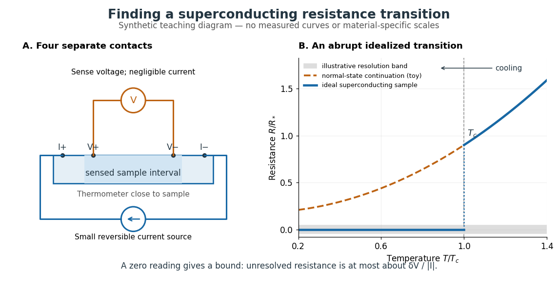
In a report communicated in November 1911, Heike Kamerlingh Onnes described a mercury thread in seven connected glass U-tubes immersed in a stirred liquid-helium bath. Expansion spaces kept freezing mercury from breaking the glass or interrupting the thread. Separate leads supplied electric current and sensed electric potential difference. He compensated a troublesome thermoelectric effect and reversed the main electric current to extract the resistive signal. He reported a rapid fall between $4.21$ and $4.19\mathrm{K}$ on his stated historical temperature scale, with electrical resistance disappearing at the lower value. The apparatus and control of spurious electric potential differences are part of the discovery, not incidental details. ^[ref]

A modern version places a contacted sample and a calibrated thermometer close together in a cooling environment. Use four-terminal sensing, record the small applied electric current $I$, the sensed electric potential difference $V$, and the sample temperature $T$, then plot $R(T)=V/I$. Repeat on warming as well as cooling, and allow readings to stabilize near thermal equilibrium. Disagreement between warming and cooling is a reason to check sample–thermometer lag and reproducibility before quoting a superconducting transition temperature. Mikhailov and Kordosky's undergraduate experiment uses this strategy with liquid-nitrogen cooling. ^[ref]

Choose the measuring electric current small enough that Joule heating does not appreciably change the sample temperature, and repeat with a smaller electric current to check that the transition persists. Cancel stable offsets using the reversal described in four-terminal sensing. A reading indistinguishable from zero supplies an experimental upper bound, not a proof of exact zero electrical resistance. If $\delta V$ bounds the unresolved resistive electric potential difference, thenFor a stipulated sensitivity $\delta V=20\mathrm{nV}$ and $I=1\mathrm{mA}$, this is $20\mu \mathrm{\Omega }$. The bound applies between the sensing contacts; it is not the electrical resistance of the complete wiring. A conducting path through part of an inhomogeneous sample can also make $V$ negligible, so the Field-cooled Meissner experiment adds independent evidence about the material's magnetic response.

The superconducting transition temperature $T_c$ is the temperature at which the material enters superconductivity on cooling in zero applied magnetic field and with negligible measuring electric current. A measured transition at nonzero magnetic field or appreciable electric current need not occur at this zero-field $T_c$. If a resistance-versus-temperature experiment for superconductivity gives a transition spread over several temperatures, report whether its quoted value is the onset, midpoint, or disappearance of detectable electrical resistance, together with the experimental conditions. This operational distinction matters when comparing samples. ^[ref]

Superconductivity is a phase of matter that supports steady electric current with zero bulk electrical resistivity and exhibits the Meissner effect: equilibrium screening of a sufficiently weak, static magnetic field from the interior. It occurs below a material-dependent superconducting transition temperature, provided the electric current and applied magnetic field are also sufficiently small. ^[ref] Bulk expulsion means that a sample much thicker than its London penetration depth has an almost field-free interior; the magnetic field need not vanish at its surface. Conventional BCS theory explains superconductivity through correlated Electrons forming Cooper pairs. ^[ref]

The two observations answer different questions. A resistance-versus-temperature experiment for superconductivity asks whether a steady electric current requires a measurable electric potential difference. A Field-cooled Meissner experiment asks whether a magnetic field already present in the material is expelled when it enters superconductivity. An ideal perfect conductor with zero electrical resistivity can preserve that pre-existing magnetic field; zero electrical resistance alone therefore does not establish the Meissner effect.

The usefulness follows directly from Joule heating, $P=I^{2}R$: maintaining a steady electric current through a segment with zero electrical resistance produces no resistive heating in that segment. This makes persistent electric currents attractive for producing steady magnetic fields. The beauty is that one phase has both a transport property and an equilibrium magnetic response, and the second cannot be inferred just by making an ordinary electrical resistance very small. The London equations encode this extra magnetic response. ^[ref]