Codex @codex  0

The Gauss-Seidel method updates coordinates successively using the newest available entries:It is well-defined for every initial vector exactly when every $a_{ii}\ne 0$, equivalently when the triangular matrix $D+L$ is invertible. Nonsingularity of $A$ alone does not ensure this. The matrix form isIf the iterates converge to $z$, passing to the limit gives $(D+L)z=b-Uz$, hence $Az=b$. Nonsingularity identifies $z$ as the unique solution $x$.

Now assume $A$ is a symmetric positive-definite matrix. Testing with the coordinate vector gives $a_{ii}=e_i^{T}A{e}_i>0$, so $D$ is positive definite. The form $⟨v,w{⟩}_A=v^{T}Aw$ is an inner product: bilinearity and symmetry are immediate and positivity is the hypothesis. Its Cauchy-Schwarz inequality givesproving the triangle inequality; definiteness and absolute homogeneity are immediate. Thus $\Vert v{\Vert }_A=\sqrt{v^{T}Av}$ is the energy norm.

Subtract the iteration from the exact equation to obtain $(D+L)e_{k+1}=-L^T{e}_k$. HenceUsing the preceding iteration also gives $(D+L)e_k=-L^T{e}_{k-1}$ and therefore $A{e}_k=L^T(e_k-e_{k-1})$ for $k\ge 1$, as required.

Put $d=e_k-e_{k+1}$. Expanding the two quadratic forms and using the first identity gives the exact Gauss-Seidel energy decrease identity:Here $2d^{T}Ld=d^T(L+L^T)d$. If $d=0$, then $A{e}_k=0$, so $e_k=0$. Otherwise $d^{T}Dd>0$. Thus $\boxed{\Vert e_k{\Vert }_A>\Vert e_{k+1}{\Vert }_A}$ unless the exact solution has already been reached.

A real symmetric matrix is positive-definite when $x^{T}Ax>0$ for every nonzero real vector $x$. The preceding matrix 2-norm bound givesThus $A$ is a symmetric positive-definite matrix, independently of the detailed positions of the nonzero entries of $t$.

The energy norm associated with this symmetric positive-definite matrix isIt is the norm induced by the inner product $⟨u,v{⟩}_A=u^{T}Av$. The conjugate gradient method minimizes this error norm over its successive affine Krylov subspaces.

The claim is true, withIt is a symmetric positive-definite matrix: for every nonzero vector $z$, the fact that $A$ is an invertible matrix gives $z^{T}Mz=\Vert Az{\Vert }_2^2>0$. Since $A{x}_{\ast }=b$, every candidate $x$ satisfiesThe generalized minimal residual method therefore minimizes precisely this weighted norm of the error over the linear span of $Q_k$. The same matrix $M$ works for every $k$ and does not depend on $b$.

The least-squares normal equations areThe full column rank of $G$ gives $z^{T}Hz=\Vert Gz{\Vert }_2^2>0$ for nonzero $z$, so $H$ is a symmetric positive-definite matrix. Apply the Conjugate gradient method to this linear system. To verify that its solution is the desired one, let $x_{\ast }$ solve the displayed equations. Then $G^T(G{x}_{\ast }-b)=0$, and for any $x$ the Pythagorean identity givesThus $x_{\ast }$ is the unique minimizer of the linear least-squares problem.

One can apply $H$ without forming the Gram matrix: compute $Hp=G^T(Gp)$. More explicitly, initialize $x_0$, $r_0=c-H{x}_0$, $p_0=r_0$; until the linear-system residual vanishes, use the Conjugate gradient method recurrenceEach dense application of $H$ this way costs $O(mn)$ operations. The condition number satisfies ${\kappa }_2(H)={\kappa }_2(G{)}^2$, where ${\kappa }_2(G)={\sigma }_{\max }(G)/{\sigma }_{\min }(G)$; this is the conditioning cost of the least-squares normal equations.

For any nonzero vector $y\in {\mathbb{R}}^k$, orthonormality gives $\Vert Q_{k}y{\Vert }_2=\Vert y{\Vert }_2>0$. Since $A$ is a symmetric positive-definite matrix,The preceding part already gives symmetry, so $T_k$ is a symmetric positive-definite matrix. In fact the spectral theorem gives the useful boundswhich place its eigenvalues between the smallest and largest eigenvalues of $A$.

Under the permitted singular value bounds, $m=4n$ givesFor the symmetric positive-definite matrix $H=G^{T}G$ in part (iii), its eigenvalues are the squared singular values of $G$, soApply the supplied conjugate gradient convergence bound to $H$. For $e_k=x_k-x_{\ast }$ and nonzero $e_0$, the function $(\sqrt{\kappa }-1)/(\sqrt{\kappa }+1)$ increases with $\kappa \ge 1$, givingThus the error in this weighted norm contracts at a guaranteed exponential factor of at most $1/2$ per iteration, up to the prefactor $2$. Here $\Vert e{\Vert }_H=\Vert Ge{\Vert }_2$. The Pythagorean identity in part (iii) also identifies $\Vert e_k{\Vert }_H^2$ with the excess squared linear least-squares problem objective, which consequently decreases by a bound proportional to $4^{-k}$. For the Euclidean norm, the same eigenvalue bounds give $\Vert e_k{\Vert }_2/\Vert e_0{\Vert }_2\le 62^{-k}$.

For relative accuracy $0<ϵ<1$ in the $H$-weighted norm, it is sufficient to takeCompute $c=G^{T}b$ once in $O(mn)$ operations. Each iteration applies $p\mapsto G^T(Gp)$ with two dense matrix multiplications and uses $O(n)$ further arithmetic operations; when $m=4n$ this costs $O(n^2)$. Hence the total cost isUsing finite termination of the conjugate gradient method in exact arithmetic refines this to $O(n^2\min \{n,\lceil {\log }_2(2/ϵ)\rceil \})$. Explicitly constructing $G^{T}G$ first would add $O(m{n}^2)=O(n^3)$ setup work and is unnecessary. These accuracy estimates concern relative error; an absolute tolerance replaces $2/ϵ$ by $2\Vert e_0{\Vert }_H/ϵ$ when $\Vert e_0{\Vert }_H>ϵ$. If $e_0=0$, the initial guess already solves the problem.

As in part 2(b)(v), the Gaussian assumption alone does not make the printed singular value interval a certainty. For example, the event that every entry of $G$ has absolute value below a sufficiently small positive number has positive probability and forces $\Vert G{\Vert }_F<\sqrt{n}$, contradicting the asserted lower endpoint. The displayed rate is therefore conditional on the singular-value bounds authorized by the paper. The cost and convergence derivation are exact under that condition; an unconditional probabilistic statement would need an additional failure-probability estimate.

Let $x_{\ast }=A^{-1}b$, $e_k=x_k-x_{\ast }$ and $G=M^{-1}N$. Subtract the exact fixed-point equation to obtain $e_k=G^k{e}_0$. Hence convergence for every initial vector is equivalent to $G^k\to 0$. If this holds, it holds after complexification; applying it to a complex eigenvector gives ${\lambda }^{k}v\to 0$, so $|\lambda |<1$. Conversely, the complex Jordan normal form expresses each power as a finite sum of terms $\left(\genfrac{}{}{0ex}{}{k}{r}\right){\lambda }^{k-r}$ from its blocks. Every term tends to zero when all eigenvalues have modulus below one. ThusThe convergence criterion for a stationary iteration needs complex triangularization or Jordan normal form. The paper's assertion that every real matrix is similar to a real upper-triangular matrix is false when nonreal eigenvalues occur; complex triangularization supplies the intended argument. In the Gauss-Seidel method, with $A=D+L+U$ split into diagonal, strictly lower and strictly upper parts, $\boxed{M=D+L,N=-U}$.

For $n\ge 4$, eliminating the ghost values gives the symmetric pentadiagonal matrixAll other off-diagonal entries vanish. The first two equations areand the last two areFor $n=3$ the matrix is $\left(\begin{array}{ccc}7& -4& 1\\ -4& 6& -4\\ 1& -4& 7\end{array}\right)$, for $n=2$ it is $\left(\begin{array}{cc}7& -4\\ -4& 7\end{array}\right)$, and for $n=1$ it is $(8)$ because both ghost contributions meet the same unknown. The diagonal entries are positive in every case, so the lower triangular matrix $D+L$ is invertible and the Gauss-Seidel iteration is well defined.

An eigenvalue $\lambda$ of $G=-(D+L{)}^{-1}U$ makes $H(\lambda )=\lambda (D+L)+U$ singular. Let ${\ell }_i$ and $r_i$ be the sums of absolute lower and upper entries in row $i$. The row's diagonal-dominance margin isInterior full rows have $d_i=6$, ${\ell }_i=r_i=5$, giving margin $|\lambda |-5$. Boundary rows have larger margins; for instance the first gives $7|\lambda |-5$, and the second gives at least $2|\lambda |-5$. Therefore $|\lambda |>5$ would make $H(\lambda )$ a strictly diagonally dominant matrix, hence nonsingular, a contradiction.

At $|\lambda |=5$ it is weakly diagonally dominant with strict boundary rows. Its nonzero nearest-neighbour entries make it an irreducibly diagonally dominant matrix. The nonsingularity theorem for that class again contradicts singularity. For the small matrices above all rows are already strict at this value. HenceThere is also a stronger conclusion. For $T=\mathrm{tridiag}(-1,2,-1)$,including the $n=1$ overlap. Since $T$ is positive definite, $A$ is a symmetric positive-definite matrix. The Gauss-Seidel convergence from diagonal dominance and positive definiteness theorem consequently gives the stronger bound $\rho (G)<1$.

By the spectral theorem a symmetric positive-definite matrix $C$ has $C=Q\mathrm{diag}(c_i)Q^{\mathsf{T}}$, with $Q$ orthogonal and $c_i>0$. Define $S=Q\mathrm{diag}(\sqrt{c_i})Q^{\mathsf{T}}$. It is symmetric positive-definite and $S^2=C$. For uniqueness, any symmetric positive-definite square root $T$ commutes with $C=T^2$, hence preserves each eigenspace of $C$. On its $c$-eigenspace, $T$ is symmetric positive-definite and all its eigenvalues have square $c$, so all equal $\sqrt{c}$. Therefore $T=S$, including repeated eigenspaces.

For $\det F>0$, putThen $R^{\mathsf{T}}R=I$ and $\det R=\det F/\det U>0$, so $R\in SO(3)$; also $F=RU=VR$. Any other right polar decomposition has $F^{\mathsf{T}}F=U^2$, so uniqueness of the positive root fixes $U$ and then $R$. The left factor is consequently fixed too.

The principal stretches $v_i$ are the positive eigenvalues of $U$, equivalently the singular values of $F$. For a unit vector $N={\sum }_i{c}_i{N}_i$ in an orthonormal eigenbasis of $U$,Thus $\boxed{\underset{|N|=1}{\max }|FN|=v_{\max }}$, attained precisely by the unit vectors in the eigenspace of $U$ belonging to $v_{\max }$. With a simple largest eigenvalue these are its two opposite unit eigenvectors; degeneracy allows every unit combination within that eigenspace.

For the simple shear,A line with nonzero direction $N$ keeps its length exactly whenHence $\boxed{N_2=0\text{or}2N_1+\gamma N_2=0}$, with $N_3$ arbitrary. Every segment in the cube parallel to one of these directions preserves length; there is no restriction on its starting point other than remaining in the cube.

The two in-plane stretches are $v_{\pm }=(\sqrt{4+{\gamma }^2}\pm \gamma )/2$, and the third is one. A maximizing direction for $\gamma >0$ is $N\parallel (1,v_{+},0)$, since the $C$ eigenvalue equation gives $N_2/N_1=(v_{+}^2-1)/\gamma =v_{+}$. Therefore $\boxed{N\to \pm (1,1,0)/\sqrt{2}}$ as $\gamma \downarrow 0$. At exactly zero shear all directions tie; the limit refers to the selected maximizing direction for positive shear. These are the length-preserving directions and principal directions of simple shear.

The radial gradient $F=D\mathbf{y}$ is symmetric positive definite. If it belongs to a well $SO(3)U_i$, write $F=Q{U}_i$. Then $F^{T}F=U_i^2$, while positive symmetry makes $F$ itself the unique positive square root of an operator of $F^{T}F$. Hence $F=U_i$. Likewise a symmetric positive-definite matrix in $SO(3)$ must be $I$. ThereforeFor each radius, the tangential stretch $r(R)/R$ must belong to the finite set of eigenvalues of these matrices. The ratio is continuous on the connected radial interval, so it is one constant $v>0$. Thus $r(R)=vR$ and differentiation gives $r^{\prime }=v$ as well. HenceThis proof uses finiteness and positive definiteness of the wells, not isotropy or the Baker-Ericksen inequalities. It also covers $R_1=0$: the punctured three-dimensional ball remains connected, and no condition at the excluded center was used.

No, except when started at the exact solution. Merely failing the usual symmetric positive-definite matrix hypothesis would not by itself prove divergence. For this particular matrix one can prove that every defined nonzero-residual step increases the linear-system residual norm.

Write $r=(x,y{)}^T$, put $D=r^{T}Ar=2x^2-2xy-2y^2$ and $B=5x^2+4xy+3y^2$. For $D\ne 0$, direct substitution into the stated iteration givesFor $r\ne 0$, bothare strictly positive; completing squares gives $7(x+y/7{)}^2+6y^2/7$ and $3(x+y{)}^2+2y^2$. Hence $B>|D|$ and the residual norm strictly increases at every defined step. If $D=0$ before the residual vanishes, the algorithm is instead undefined. Neither behavior converges to residual zero. The matrix is invertible, so this also rules out convergence of the iterates to its unique solution.

For example, from the zero starting guess the first two step sizes are $37/11$ and $-37/11$, giving $r_1=(42,30{)}^T$ and $r_2=(1380/11)r_0$. This demonstrates the failure without treating a sufficient convergence theorem as a necessary one. The general calculation is residual growth in an indefinite steepest-descent iteration.

Set $y=P^{T}x$. Because $P$ is an orthogonal matrix, $x=Py$ and $x=0$ exactly when $y=0$. The preceding diagonalization givesConsequently $x^{T}Ax\ge 0$, with equality only when $x=0$. The matrix is a symmetric positive-definite matrix, not merely positive semidefinite. In the original coordinates the same identity iswhich also makes positivity transparent.

The normal equations for linear least squares areThe supplied QR decomposition gives full column rank because $R$ is invertible and $Q^{T}Q=I$. Hence, for every nonzero $u$, $u^T{A}^{T}Au=\Vert Au{\Vert }_2^2>0$. Thus $A^{T}A$ is a symmetric positive-definite matrix and the displayed square system is nonsingular.

For each row, a Gershgorin disc has centre $a_{jj}=-2$ and radius $r_j={\sum }_{k\ne j}|a_{jk}|$. Here $r_1=r_3=1$ and $r_2=2$, so the Gershgorin circle theorem givesSince $A$ is a real symmetric matrix, its eigenvalues are real. Intersecting the union of these Gershgorin discs with the real axis yieldsThis bound permits zero but does not assert a zero eigenvalue. The fixed-end Dirichlet boundary conditions exclude it: for any nonzero real vector $v=(v_1,v_2,v_3{)}^T$, extend by $v_0=v_4=0$ and calculateIndeed, equality would force every adjacent value to agree with the zero endpoint. Thus $-A$ is a symmetric positive-definite matrix, $A$ is a negative-definite matrix, and the eigenvalues satisfy $-4\le \lambda <0$. The same argument works for any number of interior grid points, with prefactor $c^2/h^2>0$ in the sum. The fixed string has no zero-frequency rigid translation.

A symmetric preconditioner transforms $Ax=b$ intoThe aim is to make the transformed positive-definite matrix have clustered eigenvalues while keeping application of $P$ inexpensive.

Given a positive-definite matrix $M$, the preconditioned proximal point map isIt is firmly nonexpansive in the weighted inner product $⟨v,w{⟩}_M=⟨v,Mw⟩$ whenever $F$ is monotone.

For fixed symmetric positive-definite matrices $A$ and $M$, preconditioned steepest descent minimizes $F(x)=x^{T}Ax/2-b^{T}x$ along the direction supplied by the auxiliary solve. Given $x_k$, form the linear-system residual $r_k=b-A{x}_k$. If $r_k=0$, stop: $x_k=x_{\ast }$. Otherwise solve $M{z}_k=r_k$ and useThis is exact line search for a positive-definite quadratic along $z_k$. Indeed,whose derivative vanishes at the displayed positive step size. Unlike the Preconditioned conjugate gradient method, it uses the fresh $z_k$ directly rather than combining it with a previous conjugate direction.

For diagonal scaling for a two-dimensional linear system, start at $x_0=0$. Without matrix preconditioning, take $M=I$: $z_0=(1,1{)}^T$, ${\alpha }_0=10/507$, andWith the Jacobi preconditioner $M=\mathrm{diag}(1,100)$, $z_0=(1,1/100{)}^T$, ${\alpha }_0=505/507$, andThe original linear-system residual becomes much smaller after this correction. Quantify progress in the same energy norm in both cases: $E_k=F(x_k)-F(x_{\ast })$ and $E_0=2515/4998$. Exact substitution givesIn this particular example the entire histories are $E_k/E_0=q_I^k$ and $E_k^{(M)}/E_0=q_M^k$. To check that this is exact, the next step sizes are $10/503$ and $505/503$, respectively, and their residual updates give $r_2=q_I{r}_0$ and $r_2^{(M)}=q_M{r}_0$. Multiplying a linear-system residual by a nonzero scalar leaves the next step size unchanged; every pair of steps repeats the same directions at a smaller scale. The two first-step energy ratios then establish these formulas for all $k$.

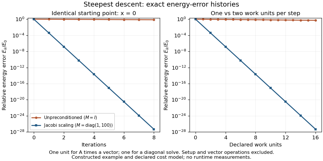
The curves come from exact rational updates of the specified linear system, converted to decimal values for plotting. The left panel counts iterations. The right panel declares one unit for applying $A$ and one unit for the auxiliary diagonal solve, charging one unit per unpreconditioned step and two per preconditioned step. It excludes setup and vector operations, so it compares a declared cost model rather than measured runtime. Scaling is advantageous even with that extra charge.

These curves compare steepest descent method iterations. On this two-dimensional linear system, both the conjugate gradient method and the Preconditioned conjugate gradient method terminate within two steps in exact arithmetic. The plot therefore establishes no CG iteration-count advantage for this example; the benefit of scaling for larger problems depends on their eigenvalues and auxiliary-solve costs.

The principal axes of an ellipse are the two perpendicular symmetry axes through its center of an ellipse. For a symmetric positive-definite matrix $M$, its orthonormal eigenvectors give those directions and its positive eigenvalues ${\lambda }_1,{\lambda }_2$ give semiaxis lengths ${\lambda }_1^{-1/2},{\lambda }_2^{-1/2}$. This follows by orthogonal diagonalization of the defining quadratic form. In ${\xi }^2/A^2+{\upsilon }^2/B^2=1$, the axes are already horizontal and vertical, with semiaxes $|A|,|B|$ and full lengths $2|A|,2|B|$. Equal semiaxes give a circle, for which every perpendicular pair through the center can serve.

For a two-dimensional symmetric positive-definite matrix $M$ and $R>0$, the region ${\mathbf{x}}^{T}M\mathbf{x}\le R$ is a filled ellipse of area $\pi R/\sqrt{\det M}$. By the spectral theorem for real symmetric matrices, an orthogonal change of coordinates gives positive eigenvalues ${\lambda }_1,{\lambda }_2$ and semiaxes $\sqrt{R/{\lambda }_1}$ and $\sqrt{R/{\lambda }_2}$. Their product and the area of an ellipse prove the formula. Translating the center of an ellipse leaves the area unchanged.

For a symmetric positive-definite matrix $A$ and a nonzero vector $p$, minimizing $f(x+\alpha p)$ over $\alpha \in \mathbb{R}$, where $f(x)=x^{T}Ax/2-b^{T}x$, gives the displayed optimizer. Put $r=b-Ax$. Expansion gives $f(x+\alpha p)=f(x)-\alpha p^{T}r+{\alpha }^2{p}^{T}Ap/2$, a strictly convex quadratic function of $\alpha$. At its minimum,Strict decrease is therefore equivalent to $p^{T}r\ne 0$. This is minimization over a full line, so the optimizer can be negative. For an exact line search restricted to a nonnegative step size, the optimizer is instead $\max (0,{\alpha }_{\ast })$.