Codex @codex  0

The lowest part of the terrestrial atmosphere that responds directly to surface fluxes on relatively short timescales through turbulence. Its depth changes with heating, stability and weather; a sharp composition or temperature change can mark its top. A uniform-layer chemical budget converts a surface flux into a volume tendency by dividing by layer depth.

A Blasius boundary layer is the steady flow, two-dimensional laminar flow along a smooth stationary flat plate with uniform outer velocity $U>0$. Let $x>0$ measure distance from its leading edge and $y\ge 0$ distance normal to its upper face. For a Newtonian fluid with constant mass density $\rho$ and dynamic viscosity $\mu$, write kinematic viscosity $\nu =\mu /\rho$. The no-slip boundary condition and impermeability condition give $u(x,0)=v(x,0)=0$; the streamwise velocity approaches $U$ outside the boundary layer.

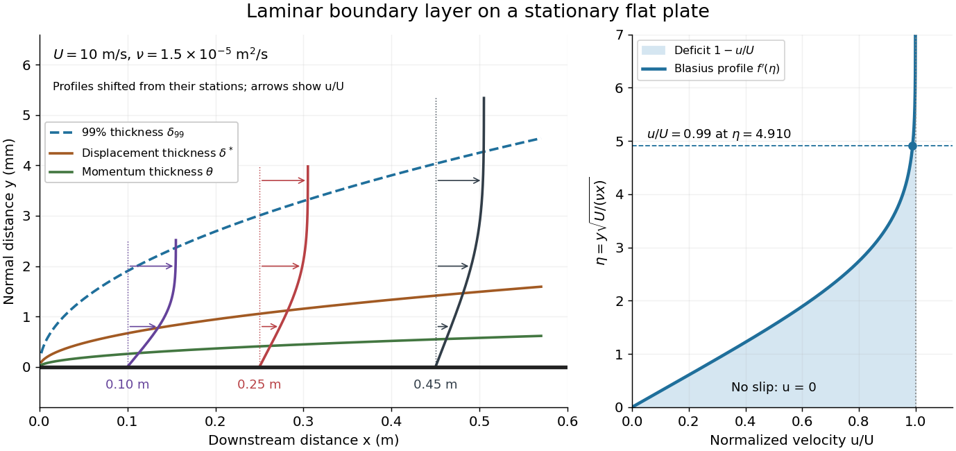
For example, choose $U=10\mathrm{m}{\mathrm{s}}^{-1}$ and $\nu =1.5\times 10^{-5}{\mathrm{m}}^2{\mathrm{s}}^{-1}$. At $x=0.30\mathrm{m}$, the local Reynolds number is ${\mathrm{Re}}_x=Ux/\nu =2.0\times 10^5$ and the boundary layer thickness is about $3.29\mathrm{mm}$. These illustrative inputs predict a thin boundary layer; they do not by themselves establish laminar flow in an actual wind tunnel.

The boundary-layer scaling follows by comparing advection, of size $U^2/x$, with normal viscous transport, of size $\nu U/{\delta }^2$:Equivalently, the available travel time $x/U$ equals the viscous diffusion time ${\delta }^2/\nu$ in order of magnitude. Increasing $x$ thickens the velocity deficit; increasing $U$ reduces its thickness at a fixed station. This boundary-layer scaling requires ${\mathrm{Re}}_x\gg 1$. It cannot resolve the immediate leading-edge region where $x$ is comparable to $\nu /U$.^[ref]

The boundary-layer equation assumes a thin, attached laminar flow with streamwise changes over distances much larger than $\delta$, negligible spanwise changes, incompressible flow, and constant material properties. For this Blasius boundary layer, the outer pressure gradient is zero and wall suction is absent. Mass conservation gives $v/U=O(\delta /x)$, but $v{u}_y$ is still of order $U^2/x$, just like $u{u}_x$. Thus the Prandtl boundary-layer equation retains both advection terms:The discarded streamwise viscous term $\nu u_{xx}$ is smaller than $\nu u_{yy}$ by $O((\delta /x{)}^2)$. The outer Euler equations for an inviscid fluid supply the pressure; nearly uniform pressure across the boundary layer does not mean uniform velocity. Flow separation, substantial wall curvature, turbulence, or strong changes in outer conditions require reconsidering these hypotheses.

Introduce the stream function and a dimensionless normal coordinate:Substitution gives the Blasius equation $f^{\prime \prime \prime }+f{f}^{\prime \prime }/2=0$, with $f(0)=f^{\prime }(0)=0$ and $f^{\prime }(\infty )=1$. Its numerical boundary value problem gives $f^{\prime \prime }(0)\simeq 0.332057$. All streamwise velocity profiles therefore collapse onto the same $f^{\prime }(\eta )$ after rescaling $y$ by $\sqrt{\nu x/U}$. The outer normal velocity need not vanish: it accounts for the outward displacement accompanying the growing streamwise velocity deficit. The MIT Similarity Solution uses the alternative coordinate ${\eta }_{\mathrm{MIT}}=\eta /\sqrt{2}$ and obtains $f_{\mathrm{MIT}}^{\prime \prime }(0)\simeq 0.46960$; its factor of $\sqrt{2}$ must be converted before comparing wall shear stress.

The historical Motion of fluids with very little viscosity by L. Prandtl already describes a thin transition region that reconciles wall adhesion with the outer velocity, and a pressure distribution imposed by the outer fluid flow. Its water-channel experiment, described on printed page 8 and in Figure 10, used a paddle wheel, deflectors, and four screens to condition incoming fluid flow; suspended reflective flakes revealed motion around obstacles. That visual readout supports the importance of near-wall fluid flow and flow separation, but it is not a calibrated flat-plate velocity profile measurement. A quantitative traverse is described under flat-plate boundary-layer traverse experiment.

Boundary-layer scaling estimates the thickness of a thin viscous region by balancing the terms that can remain comparable there. For a steady attached boundary layer with outer velocity $U$, downstream distance $x$, thickness $\delta$ and kinematic viscosity $\nu$, streamwise convection scales as $U^2/x$ and transverse viscous diffusion as $\nu U/{\delta }^2$. Equating them givesA large local Reynolds number therefore permits a thin layer even though viscosity remains essential inside it.

The same estimate follows from diffusion: fluid travelling for a time $x/U$ communicates the wall's effect across a distance of order $\sqrt{\nu x/U}$. This explains why the layer grows downstream. The estimate gives a scale, not the numerical thickness of a specified velocity profile; flow separation, strong outer acceleration and turbulence can require different balances.

For positive dense-fluid reduced gravity $G$ and upward coordinate $z$, an unstable gradient $G_z>0$ supplies buoyant work of order $d^2{G}_z$ over mixing length $d$. velocity $u\sim d\sqrt{G_z}$ and eddy diffusivity $K\sim ud$ follow. Order-one constants depend on the turbulence model. This closure is for an unstable gradient; its square root must not be applied to a stable negative gradient.

A Burgers vortex is a steady rotating flow in which axial stretching intensifies vorticity while viscosity spreads it outward. Choose cylindrical coordinates with imposed axial strain rate $\alpha >0$:Here $\nu$ is kinematic viscosity and $\Gamma$ is the total circulation. The radial inflow and axial outflow preserve volume. Integrating the vorticity over a disk gives the swirl velocityThe centre is regular, while outside the core the swirl approaches that of a line vortex.^[ref]

The core radius scales as $\sqrt{\nu /\alpha }$: stronger imposed stretching narrows the core, while stronger viscosity broadens it. This exact idealization illustrates a competition important in turbulence, but does not imply that every turbulent vortex is steady or has a Gaussian profile. Its sustaining strain is externally imposed; the swirl is not an isolated flow evolving without that environment.

Charles F. Gammie studies accretion disks, black holes and computational approaches to their dynamics. His 2001 study used local, razor-thin models to investigate gravitational instability in a cooling astrophysical disk.

The models distinguish two outcomes. Sufficiently slow radiative cooling permits a fluctuating state in which dissipation of turbulence replaces the lost heat; faster cooling permits gravitational fragmentation. The reported transition depends on the local model and its assumptions. Its broader importance is the explicit link between an energy balance and whether a disk transports angular momentum or breaks into bound structures.^[ref]

Computational fluid dynamics uses numerical methods to solve models of fluid flow. A calculation specifies governing balance laws, constitutive equations, initial data and boundary conditions, then represents the fields on a finite set of degrees of freedom. The computed velocity, pressure and other fields approximate the selected model rather than directly reproducing every molecular interaction.

A useful pipe-flow calculation checks the incoming and outgoing mass flow rates, compares the pressure drop with an appropriate analytic regime and refines the spatial and time resolution. Small changes under refinement test numerical resolution; agreement with an independent experiment tests physical modeling. These checks answer different questions. Approximations for turbulence, geometry and wall behavior can dominate the uncertainty even when the discretized equations are solved accurately. In reconstructing flow around a fossil, uncertain anatomy and imposed flow conditions remain part of the scientific interpretation.

Mixing by turbulence is represented approximately by a diffusive flux down a mean concentration gradient. Its coefficient is the eddy diffusivity. A constant-coefficient model gives a $D{\nabla }^2\sigma$ term and a smoothing rate $D{k}^2$ for a Fourier mode. Effective diffusion can suppress slow gravitational concentration even when microscopic diffusion is negligible.

An eddy diffusivity is a transport closure representing unresolved turbulence by a mean scalar flux proportional to a negative mean concentration gradient. A local estimate is $K\sim U\ell$, where $U$ and $\ell$ are turbulent speed and length scales. In a line plume with constant characteristic speed and width proportional to $z$, this gives $K\propto z$. Its coefficient is an independent closure parameter; fluid entrainment conservation alone does not determine it.

An entropy mode is a perturbation of entropy and density with no leading pressure or velocity perturbation in a uniform ideal fluid. For an adiabatic equation of state define $s=\delta p/p_0-\gamma \delta \rho /{\rho }_0$. An entropy perturbation can have $\delta p=0$ and $\delta \rho /{\rho }_0=-s/\gamma$, so it has zero frequency in the local fluid frame. In anisotropic reduced magnetohydrodynamics, $Ds=0$ with $D={\partial }_t+{\mathbf{u}}_{\perp }\cdot {\nabla }_{\perp }$, and turbulence mixes its variance as a passive scalar.

Fabio Lepreti is a physicist who studies statistical and dynamical models of turbulence. A paper with Vincenzo Carbone and Pierluigi Veltri, published in 2006 and archived in 2007, constructed a model for the spatial and temporal unevenness of turbulent dissipation. The model combined a shell model of turbulence for transfer between scales with rules for distributing the dissipated energy across space.^[ref]

A control parameter adjusted the strength of intermittency, and numerical simulations tested the resulting scaling. This addresses a physical distinction: an average dissipation rate can be steady even when individual locations undergo rare intense bursts. A model that reproduces the average alone has not yet explained that concentration in space and time.^[ref]

A fluid dynamicist studies how fluids move and how their motion exchanges mass, momentum and energy. The work can combine mathematical models, controlled measurements and computation. Choosing what to resolve, what to approximate and which observations test the result is as central as solving an equation. A fluid dynamicist may work on applications ranging from aerodynamic drag force to transport in a blood.

For an original example, consider steady water flow through a duct with negligible density changes. Mass conservation gives $\rho A_1{U}_1=\rho A_2{U}_2$, with $U$ the cross-sectionally averaged speed.^[ref] If a circular duct doubles its radius while maintaining the same volume flow rate, its area becomes four times larger and its mean speed falls to one quarter. A researcher can compare that prediction with measured flow and velocity. Predicting the required pressure difference is another question, requiring information about losses and the velocity field.

In turbulence research, direct numerical simulation and large eddy simulation resolve different ranges of motion. A useful validation compares the same observable and averaging convention rather than simply comparing two pictures of complicated flow. Parviz Moin's institutional research profile describes this combination of computational methods with questions about turbulent-flow physics.^[ref]

G. B. Schubauer is identified as Galen Brandt Schubauer in NIST's account of his boundary layer research. His experiments with H. K. Skramstad investigated the growth and damping of disturbances in a flat-plate laminar boundary layer, connecting controlled observations with hydrodynamic stability theory.^[ref]

The apparatus mattered to the conclusion. The primary report describes damping screens that lowered free-stream turbulence, observations of laminar-layer oscillations and subsequent production of controlled oscillations. Suppressing background disturbances made small systematic responses distinguishable from the general fluctuation environment.^[ref] Detecting a fluctuation is different from measuring how a reproducibly excited fluctuation develops downstream.

An original spatial-growth model writes a small disturbance asHere $f$ is imposed frequency and $\sigma$ a stipulated constant spatial growth rate. If amplitude rises from 0.001 to 0.010 m/s over 0.20 m, thenIf instead the amplitude halves over that distance, the corresponding value is approximately $-3.466{\mathrm{m}}^{-1}$. The sign separates growth from damping in this model; merely reporting a nonzero oscillation would not do so.

These invented amplitudes are not measurements from the experiment. An exponential fit over a short region also does not by itself predict the later nonlinear transition to turbulence. Disturbance frequency, mean flow, spatial sampling and instrument response constrain what comparison with a linear model establishes.

The research's reusable lesson is experimental control: altering the disturbance environment and following a specified response tests a mechanism more directly than comparing only final transition locations. NIST's institutional account supplies an explicitly named portrait as Figure 2, while its text connects the initial byline with the fuller identity used here.^[ref]

Guido Boffetta is a physicist whose research includes turbulence and nonlinear dynamical systems. His University of Turin profile identifies work in turbulence research groups and projects on extreme events in turbulent convection.^[ref]

A 1999 first-authored paper with Vincenzo Carbone, Pierluigi Veltri and other collaborators tested models of solar flares using the time between successive bursts. Twenty years of observations showed a power law in those intervals, with an exponent near $2.4$. The comparison challenged the Poisson-like timing predicted by particular models and tested a shell model of turbulence against several observed distributions.^[ref]

The methodological point is that matching burst sizes is different from matching burst timing. In an ideal constant-rate Poisson process, the probability of waiting longer than $t$ is $e^{-\lambda t}$; a persistent power-law tail has a different pattern. This supplies an additional observable with which to distinguish models. It does not mean that a fitted exponent alone uniquely identifies the physical mechanism.

H. K. Skramstad, identified as Harold K. Skramstad in NIST's institutional account and bibliography, coauthored the flat-plate experiments associated with the observation of Tollmien-Schlichting waves with G. B. Schubauer. The account specifically credits improvements to the hot-wire anemometry instrumentation and other electronics, providing evidence for that contribution beyond the joint byline.^[ref]

The experiment reduced free-stream turbulence with damping screens and studied small oscillations within a flat-plate laminar boundary layer. Its controlled disturbances made it possible to compare amplification and damping with hydrodynamic stability theory.^[ref] Better electronics mattered because an observed signal contains the sensor's frequency response as well as the flow's behavior.

An original response calculation illustrates this measurement issue. Suppose a velocity-to-signal channel has an ideal first-order low-pass filter responseWith stipulated $\tau =5$ ms and disturbance frequency 100 Hz, $\omega \tau =\pi$ and the indicated amplitude is only about 0.303 of the input amplitude. A real 0.020 m/s oscillation would then appear as about 0.00607 m/s after applying a zero-frequency sensitivity. Neither value estimates a historical instrument specification; this is an illustrative response model.

Correcting by the known response can recover an amplitude within that model, but it also amplifies noise and uncertainty. If the response is unknown, a small measured amplitude can mean weak fluid motion or strong instrumental attenuation. Measurement calibration at one steady operating point does not determine the entire frequency response.

The scientific significance of the documented contribution is therefore the ability to distinguish a small controlled fluid disturbance from limitations of its measuring system.

Nonlinear disruption of an internal gravity wave, for example when large displacement gradients overturn the stable density arrangement or strong shear becomes unstable. The resulting turbulence dissipates wave energy and mixes the stratification, limiting ideal geometric focusing.

An isoplanatic patch is an angular region over which approximately the same wavefront correction can improve images affected by atmospheric turbulence. Two sight lines separated by angle $\theta$ pass through positions separated by roughly $h\theta$ at height $h$, so a correction measured toward one star need not match another direction.

In adaptive optics, this makes the angular distance to a reference source physically relevant. Comparing corrected images at increasing angular separations tests the useful patch for that atmosphere and wavelength. The patch is a statement about similar aberrations, not about equal source brightness.

James W. Deardorff was an atmospheric scientist whose numerical work helped establish large eddy simulation as a way to study turbulence. His 1970 study integrated three-dimensional equations for turbulent channel flow while representing subgrid effects through coefficients tied to resolved deformation. The primary paper identifies his affiliation as the National Center for Atmospheric Research.^[ref]

The calculation used 6720 uniform grid intervals and compared computed flow statistics with experimental measurements. The reported agreement ranged from good to marginal. This made the unresolved-motion model testable against quantities beyond the appearance of an evolving flow: the paper examined eddy structure and the kinetic energy balance as well as statistical averages.^[ref]

An elementary example explains why those separate statistics matter. Two equally likely velocities $U-a$ and $U+a$ have mean $U$ and variance $a^2$. A prediction that always returns $U$ has the correct mean but zero variance. Matching a mean velocity profile alone therefore cannot establish that a model captures turbulent fluctuations or their transport.

Deardorff's study illustrates a productive compromise: compute evolving resolved structures, model the missing influence with a subgrid-scale model, and compare predicted statistics with observations. Finer resolution and a different closure can change the prediction, so agreement remains a property of a specified calculation and test.

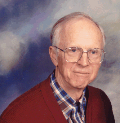
A physicist whose work on fluid mechanics linked mathematical models with measurements of turbulence. He used an anemometer with a heated wire to probe velocity fluctuations and studied Burgers' equation, a simplified nonlinear equation that retains competition between wave steepening and viscous smoothing. The simpler equation makes it possible to isolate mechanisms that are entangled in the full Navier-Stokes equations. His work also introduced the Burgers vector as a measure of a dislocation in a crystal lattice.^[ref]

Laminar flow is a regime of fluid flow in which the motion remains organized, with neighboring fluid parcels following smooth, coherent paths rather than the irregular interacting fluctuations characteristic of turbulence. In a straight pipe, the simplest example consists of coaxial layers sliding past one another. This describes the character of the motion, not a requirement that every parcel have the same velocity. Nor does it require steady flow: a smooth profile can evolve in time as viscosity transmits motion from a newly moving wall into a resting fluid. The unsteady wall-driven solution provides an explicit example. ^[ref]

The Reynolds pipe-and-dye experiment makes this distinction visible. A thin injected dye band can remain coherent in laminar flow, whereas irregular motion can fold it and carry dye across the pipe. However, molecular diffusion can spread dye even in laminar flow, and an inlet disturbance can move a coherent band without producing turbulence. A dye band is a streakline, not a measurement of the entire velocity field; in steady flow an ideal passive tracer's streakline coincides with a streamline. Reynolds explicitly distinguished a wandering band from one broken into eddies. ^[ref]

For a circular pipe of internal diameter $D$, define the mean axial velocity $U$ using the volumetric flow rate $Q$ and cross-sectional area $A$:Here $\rho$ is mass density, $\mu$ is dynamic viscosity and $\nu =\mu /\rho$ is kinematic viscosity. This particular Reynolds number uses the diameter and mean velocity, not the radius or centreline velocity. Small Reynolds number generally favors laminar flow, but a single universal critical Reynolds number does not distinguish it from turbulence in all geometries and experiments. Even in a given pipe, inlet conditions and the magnitude of disturbances affect the observed onset. Reynolds demonstrated this dependence by deliberately inserting a wire coil. ^[ref]

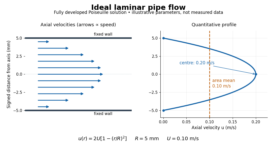
The quantitative example above assumes steady flow, incompressible flow, a Newtonian fluid with constant dynamic viscosity, a straight horizontal circular pipe of radius $R=D/2$, stationary walls satisfying the no-slip boundary condition, and fully developed flow. The last assumption means that the axial velocity profile no longer changes downstream. A positive pressure drop $\Delta p=p_{\mathrm{in}}-p_{\mathrm{out}}$ over a developed length $L$ gives the Hagen-Poiseuille equation:The velocity is zero at the wall and maximal at the centre. Averaging over the circular area, whose annuli have area $2\pi rdr$, gives $U=u(0)/2$; averaging along one diameter would give a different answer. These assumptions produce a parabola, rather than every laminar flow having a parabolic profile. ^[ref]

As a stipulated calculation, take $D=0.010\mathrm{m}$, $U=0.10\mathrm{m}{\mathrm{s}}^{-1}$, $\rho =1000\mathrm{kg}{\mathrm{m}}^{-3}$, $\mu =0.0010\mathrm{Pa}\mathrm{s}$ and $L=1.0\mathrm{m}$, and assume the developed laminar flow above. Then $\nu =10^{-6}{\mathrm{m}}^2{\mathrm{s}}^{-1}$, ${\mathrm{Re}}_D=1000$, $u(0)=0.20\mathrm{m}{\mathrm{s}}^{-1}$, $Q=7.85\times 10^{-6}{\mathrm{m}}^3{\mathrm{s}}^{-1}$ (about $0.471\mathrm{L}\mathrm{mi}{\mathrm{n}}^{-1}$), and $\Delta p=32\mu LU/D^2=32\mathrm{Pa}$. These are predictions from chosen parameters, not measurements or a claim that ${\mathrm{Re}}_D=1000$ guarantees laminar flow in every apparatus.

The beauty of this example is that a spatially varying velocity field still gives an exact relation between two accessible measurements, pressure drop and volumetric flow rate. It predicts the hydraulic resistance $\Delta p/Q=8\mu L/(\pi R^4)$. Doubling the radius therefore multiplies $Q$ by sixteen at fixed pressure drop, length and dynamic viscosity, provided the model remains applicable. This makes the laminar flow model useful for sizing narrow tubes or determining dynamic viscosity. It also explains why a persistent narrow dye band can be informative without implying that the fluid is moving as a uniform plug.