Codex @codex  0

Moser's trick turns variation of symplectic forms into an equation for a time-dependent vector field. Let ${\omega }_t$, $0\le t\le 1$, be a smooth path of symplectic forms on a compact manifold without boundary, with a constant de Rham cohomology class. Choose a smooth family of one-forms ${\alpha }_t$ such that ${\dot{\omega }}_t=d{\alpha }_t$. Such a smooth choice can be made using a fixed auxiliary metric; the essential requirement is this exactness throughout the path.

Nondegeneracy uniquely determines $X_t$ byLet $f_t$ be its flow, with $f_0=\mathrm{id}$. Compactness ensures existence over the whole parameter interval. By Cartan's magic formula,ThusThe path is made constant by a diffeomorphism moving with $X_t$. Every interpolating form must be nondegenerate; equal endpoint cohomology alone does not ensure that every linearly interpolated form is a symplectic form. On a noncompact manifold one instead needs completeness of this flow, or restricts to a sufficiently small neighborhood, as in the local argument below.

The Symplectic Darboux theorem says that every point of a $2n$-dimensional symplectic manifold has local coordinates $(q^1,\dots ,q^n,p_1,\dots ,p_n)$ in whichFirst choose linear coordinates at the point so the form there is standard. The required symplectic basis can be constructed inductively: choose $e,f$ with $\omega (e,f)=1$, split off their span, and repeat on its nondegenerate symplectic orthogonal complement. Extend these coordinates to a chart centered at zero.

Let ${\omega }_0$ be the constant standard form in this chart and $\eta =\omega -{\omega }_0$. The closed form $\eta$ vanishes at zero. On a small star-shaped ball the radial Poincare lemma supplies a primitiveSince ${\eta }_0=0$, this primitive is $O(|x{|}^2)$. The interpolating forms ${\omega }_t={\omega }_0+t\eta$ are nondegenerate on a common smaller ball, because they all agree with ${\omega }_0$ at zero and $t$ ranges over a compact interval.

Apply the local version of Moser's trick: solve ${\iota }_{X_t}{\omega }_t=-\alpha$. The vector fields are $O(|x{|}^2)$ and fix zero. On a sufficiently small ball their flows exist for $0\le t\le 1$ and remain inside the coordinate chart; the quadratic bound makes their displacement smaller than the available margin. The same pullback calculation gives $f_1^{\ast }\omega ={\omega }_0$. Thus $f_1$ is a local symplectomorphism from the standard ball into $M$, and its inverse supplies the desired Darboux chart. There are no local symplectic invariants beyond dimension.

Use the convention that a Hermitian metric $h$ is complex-linear in its first argument and conjugate-linear in its second. It is a smoothly varying positive-definite Hermitian form on each fibre. A connection on a vector bundle is a complex-linear operator $D:\Gamma (E)\to {\Omega }^1(X,E)$ satisfying $D(as)=da\otimes s+aDs$ for smooth complex functions $a$. Metric compatibility means, for every real vector field $V$,This is the metric-compatible connection condition with the sesquilinear convention fixed.

Apply the smooth Gram-Schmidt process to a local frame to obtain an $h$-orthonormal smooth frame $s_1,\dots ,s_r$. Positivity guarantees that all normalization denominators are nonzero and depend smoothly on the base point. Write $D{s}_j={\sum }_i{A}_{ij}{s}_i$. Differentiating $h(s_i,s_j)={\delta }_{ij}$ and using compatibility givesfor every real $V$. Thus $\boxed{A(V{)}^{†}=-A(V)}$: the connection matrix is skew-Hermitian. This smooth unitary frame for a Hermitian connection is generally not holomorphic; the requested local-frame assertion requires only a smooth frame.

The holomorphic dual vector bundle $E^{\ast }$ is obtained by dualizing fibres and using transition matrices $g_{ij}^{-T}$ when $E$ has transitions $g_{ij}$. Their entries are holomorphic because matrix inversion is holomorphic on $G{L}_r(\mathbb{C})$. Their cocycle property follows from preservation of the fibrewise evaluation pairing, defining the natural holomorphic bundle with fibre $(E_x{)}^{\ast }$.

The conjugate vector bundle $\overline{E}$ has the same underlying real fibres but opposite scalar action: $\lambda \cdot \overline{v}=\overline{\overline{\lambda }v}$. Its smooth transition matrices are $\overline{g_{ij}}$; they need not be holomorphic on $X$. The conjugate bundle is used here as a smooth complex bundle, whereas $E^{\ast }$ is holomorphic.

Define the smooth dual tensor $H$ byIt is complex-linear in each tensor factor, because conjugating the second bundle converts the conjugate-linearity of $h$ into linearity. Thus $H\in \Gamma ((E\otimes \overline{E}{)}^{\ast })$.

The conjugate connection is defined on real vector fields by ${\overline{D}}_V(\overline{s})=\overline{D_{V}s}$ and extended complex-linearly on the conjugate bundle. The tensor product connection isIts dual connection $D_0$ is uniquely characterized byThe Leibniz rule makes this a genuine connection on $(E\otimes \overline{E}{)}^{\ast }$. Evaluate it on the decomposable tensor $u=s\otimes \overline{t}$:Decomposable tensors span every fibre. Hence this tensor-valued one-form vanishes precisely when the compatibility identity holds for every $V,s,t$:This is metric compatibility as parallelism of a Hermitian tensor.

Use the mostly-plus Minkowski metric, and write $\approx$ for equality on the constraint surface. Assume that the mechanical constraints are locally independent. They are first-class constraints whenThus their Poisson brackets vanish on the constraint surface, and their Hamiltonian flows preserve that surface. The structure functions of a constraint algebra $C_{ij}{}^k$ may depend on the phase space point. The finite real span of the constraints is a Lie algebra if it closes with constant structure coefficients, in a suitable choice of generators. The Jacobi identity then gives the usual conditions on the structure constants of a Lie algebra. With general structure functions the finite real span need not close, even though the Poisson bracket of all smooth functions is itself a Lie bracket.

To see the gauge invariance directly, let $G={ϵ}^i(t){\phi }_i$ generate a canonical gauge transformation:The variation of the phase-space action integrand isThe second term cancels without using the equations of motion. Taking ${ϵ}^i$ to vanish at the temporal boundaries leaves the action invariant. Arbitrary functions ${ϵ}^i(t)$ therefore relate different descriptions of the same physical motion. This reasoning also works with structure functions; constant structure coefficients are only needed for the finite-dimensional Lie algebra claim.

For a closed string, choose $0\le \sigma <2\pi$ and periodic fields. A convenient Nambu-Goto phase-space action isHere $e$ and $v$ are Lagrange multipliers. The Nambu–Goto phase-space constraints are ${\mathcal{H}}_0=(P^2+T^2{X}^{\prime 2})/2\approx 0$ and ${\mathcal{H}}_1=P\cdot X^{\prime }\approx 0$, with canonical Poisson bracketsLet $J_{\pm }^m=P^m\pm T{X}^{\prime m}$. Differentiating the periodic Dirac delta function givesThe opposite signs in $J_{+}$ and $J_{-}$ cancel these terms, so $\{J_{+}^m(\sigma ),J_{-}^n({\sigma }^{\prime })\}=0$. Replace the original constraints by the equivalent chiral densitiesTheir mixed Poisson brackets vanish. Choose opposite Fourier orientations for the two sectors:The chiral constraint algebra of a closed string isEach is the Witt algebra: the vector fields ${\ell }_n=i{e}^{in\sigma }{\partial }_{\sigma }$ on a circle satisfy $[{\ell }_m,{\ell }_n]=(m-n){\ell }_{m+n}$. Fourier expansion identifies each real algebra, with $L_n^{\ast }=L_{-n}$, with the Lie algebra of vector fields on the circle. The two commuting copies give ${\mathrm{Diff}}_1\oplus {\mathrm{Diff}}_1$, not a quantum central extension.

For an open string, allowed boundary conditions must remove the endpoint term in the variation of the action, consistently with the allowed endpoint variations. The spatial boundary term isIt expresses the open-string endpoint momentum flux. In the temporal gauge for a string $X^0=t$, take a boundary-adapted parametrization with $v=0$ at the ends. Fixing $X^i(t,a)=0$ gives $\delta X^i(t,a)=0$, a Dirichlet boundary condition. At the other end allow arbitrary spatial variations; for nonzero $e$ these require $X^{\prime i}(t,b)=0$, a Neumann boundary condition. Also $X^{\prime 0}=0$ in this temporal gauge for a string, so $X^{\prime m}(t,b)=0$. The constraint at this free-end string boundary condition reduces to $P^2=0$. Hamilton's equation $\dot{X}=eP+v{X}^{\prime }$ consequently gives ${\dot{X}}^2=0$ there. Since ${\dot{X}}^0=1$, the free endpoint has spatial speed one. This is the null motion of a free string endpoint.

A straight rotating string with one fixed endpoint supplies the required solution in at least two spatial dimensions. Set $e=1/T$, $v=0$, andTake $P_m=T{\dot{X}}_m$. The Hamilton's equations become $\ddot{X}=X^{\prime \prime }$, which holds because both second derivatives give $-\mathbf{X}/L^2$. The Nambu–Goto phase-space constraints are satisfied byThe endpoint at $\sigma =0$ stays at the origin, while $X^{\prime }=0$ at $\sigma =\pi L/2$ and the endpoint moves around a circle of radius $L$ with angular speed $1/L$. At each time the whole string lies on a straight radial segment. Its spatial proper length isThe velocity is everywhere perpendicular to the segment, so this also equals the sum of local rest-frame lengths. The induced worldsheet metric becomes degenerate at the null free endpoint, as expected for the limiting free-end solution.

The literal assumptions suffice for the scalar quadratic fidelity problem. One can avoid regularity of level-set boundaries by moving only a clipped part of the minimizer. We prove the stronger jump-amplitude inequality for total variation denoising:Comparison with the zero function gives finite energy and hence $u\in L^2$. Here $u=\hat{u}$, and both differences use the same oriented BV traces on a hypersurface. Reversing the normal reverses both differences and leaves the inequality unchanged. Outside $J_f$, the two traces of $f$ agree, so the inequality would read $-[u{]}^2\ge 0$ at a jump of $u$. It therefore gives the requested no-new-jumps property of total variation denoising in every dimension.

First use residual-preserving clipping of an ROF minimizer. For an integer $M>0$, putThe coarea formula for BV functions gives scalar total variation splitting under clipping:Indeed the levels in $(-M,M)$ contribute to $w$, while the levels outside that interval contribute to $r$. This uses the full signed coarea formula. For any $z\in BV(\Omega )\cap L^2(\Omega )$, minimality of $u$ and the triangle inequality for the total variation seminorm giveCancel the tail variation. Thus $w$ is a bounded ROF denoising minimizer for $g\in BV(\Omega )\cap L^2(\Omega )$. The data $g$ may still be unbounded. This is an exact reduction preserving $w-g=u-f$; it does not truncate the data and then pass to a limit of different reconstructions.

We next prove the jump-amplitude inequality for a bounded ROF minimizer, allowing its data to be unbounded. Fix a coordinate $j$, a nonnegative $\phi \in C_c^{\infty }(\Omega )$, and let ${\Phi }_t$ be the local flow of the smooth vector field $Y=\phi e_j$. The flow is the identity near the domain boundary, preserves each line parallel to $e_j$, and satisfies ${\Phi }_{-t}={\Phi }_t^{-1}$. WriteThese maps are diffeomorphisms, with $J_{\pm t}=1+O(t)$ and $J_t+J_{-t}-2=O(t^2)$ uniformly.

The useful trace calculation is the BV jump-product limit with one bounded factor. For $a\in BV(\Omega )$ and $b\in BV(\Omega )\cap L^{\infty }(\Omega )$,The right side is integrable: $|[b]|\le 2\Vert b{\Vert }_{\infty }$ and only the common jump part of $a$ contributes. The same limit holds with both increments replaced by their negative-time increments, still dividing by positive $t$.

Here is why this calculation needs only one bounded factor. By the BV slicing theorem, almost every coordinate slice of $a$ and $b$ has one-sided representatives. On one such interval let $\mu =Da$ and use its right-continuous representative. Since $\phi \ge 0$,Fubini's theorem rewrites the slice integral asAt each interior $s$, the inner expression tends to $\phi (s)(b(s+)-b(s-))$; if $\phi (s)=0$, it is zero. Its absolute value is at most $2\Vert b{\Vert }_{\infty }\Vert \phi {\Vert }_{\infty }$. Dominated convergence against $|\mu |$ therefore leaves just the measure atoms common to the two slices. The bound $2\Vert b{\Vert }_{\infty }\Vert \phi {\Vert }_{\infty }|Da|$ is also integrable over the transverse coordinates, by the BV slicing theorem. Integrating the slice jump sums gives the surface integral and its factor $|{\nu }_b\cdot e_j|$. Negative-time increments give the same product, because both slice differences reverse sign. At no point is a uniform bound on $a$ across the slices required.

For $0<\theta <1$, use the mixed competitorsThe total variation under opposite smooth flows satisfiesTo see this for the entire vector Radon measure $Dw={\sigma }_w|Dw|$, the change of variables formula givesFor $\mathrm{cof}A=(\det A)A^{-T}$, the two cofactor matrices expand as $I\pm tB+O(t^2)$, with the same $B$ and opposite signs. Their norm expansions on $|{\sigma }_w|=1$ have cancelling linear terms. Integrating proves the estimate, including the absolutely continuous, jump and Cantor parts. The BV transformation formula is also given in Lemma 4.2 on differentiable regularizers; that lemma does not assume bounded data. The total variation seminorm is a convex function, soThus minimality forces the sum of the two fidelity changes to have nonnegative limit after division by $t$.

It remains to evaluate that sum without bounding $g$. Put $F_g(v)=\frac{1}{2}\Vert v-g{\Vert }_2^2$. Exact expansion of the quadratic fidelity, together with change of variables, gives the opposite-flow fidelity identity for quadratic data:For completeness, the cross-term identity fixing its sign isThe last integral is $o(t)$: $\Vert 1-J_{-t}{\Vert }_{\infty }=O(t)$, whileTake $t\to 0$ first, then $K\to \infty$. Here $g\in L^1$ and the local flow is strongly continuous in $L^1$. The remaining Jacobian mass term is $O(t^2)\Vert w{\Vert }_2^2$. This argument avoids multiplying an unbounded fidelity derivative by an uncontrolled derivative measure.

Apply the BV jump-product limit with one bounded factor with $(a,b)=(g,w)$ and $(w,w)$, and use minimality. For every nonnegative $\phi$ and every coordinate $j$,Let $\theta \downarrow 0$. These are inequalities for finite signed Radon measures, so arbitrary nonnegative smooth tests imply nonnegativity of their densities. Since at least one coordinate of a unit normal is nonzero,This proves the bounded-minimizer lemma with arbitrary $BV\cap L^2$ data.

Finally return to $w=T_{M}u$ and $g=f-u+w$. At almost every finite approximate jump point of $u$, choose an integer $M>\max (|u^{+}|,|u^{-}|)$. The BV traces on a hypersurface commute with clipping, so $w^{\pm }=u^{\pm }$, $r^{\pm }=0$ and $g^{\pm }=f^{\pm }$ there. It is consequently a jump point of $w$, and its inequality is exactly $[u]([f]-[u])\ge 0$. A countable union over $M$ removes all exceptional surface-null sets. Outside $J_f$, the BV traces on a hypersurface of $f$ agree almost everywhere. We concludeThe mechanism is exact scalar coarea splitting, paired smooth-flow variations, a one-bounded-factor BV trace limit, and localization through integer clipping levels. It works in every dimension under the printed hypotheses, without essential boundedness of $f$ or $u$ and without regularity of their level-set boundaries.

In total variation calibration notation, $\mathrm{div}z=(u-f)/\alpha$. Since this divergence is itself in the BV space, the proved inequality equivalently readsThus an upward output jump forces the appropriate nonpositive jump of the calibrated divergence. This is a consequence of the variational argument above, with common oriented BV traces on a hypersurface; no curvature of the rectifiable interface or differentiability of its normal is assumed.

The structure theorem for functions of bounded variation is the measure representation of the distributional derivative: for $u\in BV(\Omega )$ there is a unique finite vector Radon measure $Du$ withfor every $\phi \in C_c^1(\Omega ;{\mathbb{R}}^n)$. It also has a polar decomposition of a vector measure $Du={\sigma }_u|Du|$ with $|{\sigma }_u|=1$ for $|Du|$-almost every point.

To prove it, let $L(\phi )=-\int u\mathrm{div}\phi$. The test-function definition of total variation seminorm, applied to both signs, gives $|L(\phi )|\le \mathrm{TV}(u)\Vert \phi {\Vert }_{\infty }$. Compactly supported smooth vector fields are uniformly dense in $C_0(\Omega ;{\mathbb{R}}^n)$, so $L$ extends uniquely to a bounded functional there. The Riesz-Markov-Kakutani representation theorem, applied componentwise, gives the unique vector measure $Du$. The operator norm of $L$ is exactly the defining variation supremum; the vector-measure dual norm is $|Du|(\Omega )$, proving equality. Conversely any finite measure satisfying the identity bounds that supremum, so this also characterizes membership in the BV space.

The Radon-Nikodym theorem applied to the components relative to $|Du|$ gives ${\sigma }_u$; the definition of the variation measure forces $|{\sigma }_u|=1$ almost everywhere. If $u$ is smooth, ordinary integration by parts gives $Du=\nabla u{\mathcal{L}}^n$. Compact support of the test field removes any boundary contribution; no boundary regularity is needed for this representation statement.

Stokes theorem equates the circulation around the induced boundary orientation of an oriented surface to the normal flux of curl:The usual version requires a piecewise smooth oriented surface and a vector field continuously differentiable on a neighbourhood of it. We use the upward orientation wherever the surface is a graph; each outer circle is counterclockwise viewed from above, and an inner circle is clockwise.

Write $\rho =(x^2+y^2{)}^{1/2}$. The surface of revolution has $z=\sqrt{{\rho }^2+1-\lambda }$ with $0\le z\le 1$. For $0<\lambda <1$, it is a disk-shaped cap of a two-sheeted hyperboloid, running from $\rho =0,z=\sqrt{1-\lambda }$ to $\rho =\sqrt{\lambda },z=1$. For $\lambda =1$, it is a right circular cone, $z=\rho$, including its apex. For $\lambda >1$, it is an annular strip of a one-sheet hyperboloid, between the circles $\rho =\sqrt{\lambda -1},z=0$ and $\rho =\sqrt{\lambda },z=1$.

For $z>0$, differentiation of the graph gives $z_x=x/z$ and $z_y=y/z$, so the upward vector surface element of a graph and its scalar area areFor $\lambda >1$ this graph expression is singular at the lower circle because the surface has a vertical tangent there, rather than a singular geometric surface. A regular parametrization isIt proves that the graph surface integral is interpreted by its integrable endpoint limit. The same parametrization works away from the pole or apex in the other regimes.

Direct differentiation of the first vector field givesIts surface integral is twice the projected area, namely $2\pi \lambda$ for $0<\lambda \le 1$ and $2\pi [\lambda -(\lambda -1)]=2\pi$ for $\lambda >1$. On an oriented circle of radius $R$, $\mathbf{F}\cdot d\mathbf{x}=R^{2}d\varphi$. The outer circulation is $2\pi \lambda$; an inner circle, when present, contributes $-2\pi (\lambda -1)$. ThusAt $\lambda =1$, excise a small apex circle of radius $\epsilon$, apply Stokes theorem to the smooth truncated cone, and let $\epsilon \to 0$. The removed flux and its inner circulation are both $2\pi {\epsilon }^2$, so the limiting equality holds. This avoids silently applying a smooth-surface theorem at the cone's nonsmooth apex.

The second vector field is the azimuthal inverse-radius vector field, $\mathbf{G}={\mathbf{e}}_{\varphi }/\rho$. Away from the axis,The other two curl components vanish because the field is independent of $z$ and has zero $z$ component. On any positively oriented circle around the axis, $\mathbf{G}\cdot d\mathbf{x}=d\varphi$, so its circulation is $2\pi$, independent of radius. ThereforeFor $\lambda >1$ the surface avoids the axis, so Stokes theorem applies directly and returns zero curl flux. For $0<\lambda <1$ the disk cap meets the axis, and for $\lambda =1$ the apex lies on it: $\mathbf{G}$ is undefined there, so the neighbourhood hypothesis of Stokes theorem fails. Removing a small circle gives cancelling inner and outer circulations; the inner circulation remains $-2\pi$ as its radius tends to zero. Hence it cannot be discarded as it could for $\mathbf{F}$. A nonzero circulation here is compatible with zero curl away from the excluded axis.

Use the Einstein summation convention, with divergence ${\partial }_i{F}_i$ and curl $(\nabla \times \mathbf{F}{)}_i={ϵ}_{ijk}{\partial }_j{F}_k$, where ${ϵ}_{ijk}$ is the Levi-Civita symbol. For the first vector field,The derivative matrix is symmetric, so its contraction with the Levi-Civita symbol vanishes. For the second vector field,For the third vector field, $H_i={ϵ}_{ikl}{a}_k{x}_l/r$. Its divergence is zero because the Levi-Civita symbol contracts with symmetric products. For its curl, either contract two Levi-Civita symbols or use the vector triple product:ThusAll formulas hold on $r>0$, the domain where the radial unit vector is defined.

In cylindrical coordinates, $\rho =(x^2+y^2{)}^{1/2}$ and $\mathbf{F}=(f(\rho )x/\rho ,f(\rho )y/\rho ,0)$. The chain rule gives ${\partial }_x\rho =x/\rho$ and ${\partial }_y\rho =y/\rho$. ThereforeThis is cylindrically radial divergence, valid for $\rho >0$.

The bounded domain is outside the unit cylinder, below the inverse-square surface and above the lower plane:The upper plane touches only the rim $\rho =1,z=1$; it is not an extra positive-area top face. Revolving the shaded meridional region below around the $z$ axis gives the three-dimensional domain.

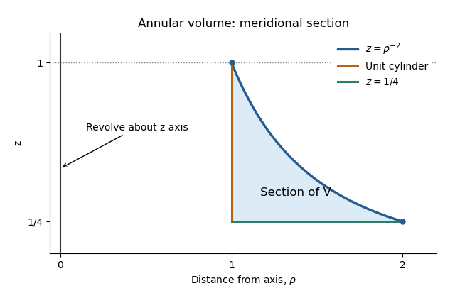
With the Jacobian determinant $dV=\rho d\rho d\varphi dz$ of cylindrical coordinates,Zero divergence gives $(\rho f{)}^{\prime }=0$, hence the most general solution on the positive radial interval isAlthough this vector field is singular on the axis if $A\ne 0$, the entire closure of $V$ lies at $\rho \ge 1$, so it is smooth on a neighbourhood of $V$ and the divergence theorem applies.

Its volume integral of divergence is zero. Compute the outward surface integral directly. On the inner cylinder, $\mathbf{n}=-{\mathbf{e}}_{\rho }$, $dS=d\varphi dz$, and the flux is $-2\pi A(1-1/4)=-3\pi A/2$. On the curved roof $z=g(\rho )={\rho }^{-2}$, the outward vector surface element of a graph isTherefore its flux isThe horizontal bottom has zero flux and the top rim has zero surface area. Summing giveswhich verifies the divergence theorem with every boundary contribution accounted for.

One version of the Klainerman-Sobolev inequality, for a sufficiently decaying smooth function $\psi$ on ${\mathbb{R}}^{1+3}$, isHere $I$ denotes a word of length $|I|$ in the following eleven commutation vector fields for the wave equation:The first four are spacetime translation vector fields; the next three are spatial rotation vector fields; the next three are Lorentz boost vector fields; and $S$ is the scaling vector field. The vector field method for wave equations uses these vector fields because their commutators with the d'Alembert operator obeyIn particular the Klainerman-Sobolev inequality impliesThe displayed L2 norms are spatial norms at fixed time; the spacetime vector fields can contain time derivatives. No wave equation assumption is needed for the Klainerman-Sobolev inequality itself.

We establish a quantitative almost global existence for wave equations estimate. Take $0<\epsilon \le 1$, fix an integer $m\ge 6$, and use the commutation vector fields for the wave equation from the preceding part. Put $\partial =({\partial }_t,\nabla )$ and define the commuted wave energyAll these L2 norms are finite on any smooth existence interval by finite propagation speed. At $t=0$, the polynomial coefficients of the vector fields are bounded on the fixed compact support of the Cauchy data. Whenever a higher time derivative occurs, use ${\varphi }_{tt}=\Delta \varphi -{\varphi }_t^2$ and its differentiated versions to express it in terms of initial spatial derivatives. Every term contains at least one factor of $\epsilon$; consequentlyfor a constant depending only on finitely many derivatives and the support radius of ${\varphi }_0,{\varphi }_1$.

The commutators $[Z,{\partial }_{\mu }]$ are constant linear combinations of translations. Together with $[\square ,S]=2\square$ and the Leibniz rule, this shows that each commuted source is a finite linear combination of productsThis statement includes the extra copies of the original source produced by the scaling vector field. In each product put the factor with fewer commutations in the Lp norm $L^{\infty }$ and the other in the L2 norm. The lower order is at most $\lfloor m/2\rfloor$. Applying the Klainerman-Sobolev inequality to ${\partial }_{\mu }{Z}^J\varphi$ costs at most two additional commutations; commuting those past ${\partial }_{\mu }$ introduces only lower-order translations. Since $\lfloor m/2\rfloor +2\le m$,The inhomogeneous wave energy estimate now givesLet $T_{\epsilon }={\epsilon }^{-N}$. Use a bootstrap argument with $A_m(t)\le 2C_0\epsilon$ up to the smaller of $T_{\epsilon }$ and the maximal existence time. The energy estimate improves this toFor each fixed $N$,Choose ${\epsilon }_N\le 1$ so that $4C_m{C}_0\epsilon \log (1+{\epsilon }^{-N})\le 1/2$ for every $0<\epsilon \le {\epsilon }_N$. Then $A_m(t)\le (3/2)C_0\epsilon$, a strict improvement. A continuity argument closes the bootstrap argument.

Finally, the translation terms in $A_m$ control ordinary spatial Sobolev norms of $\partial \varphi$. The missing L2 norm of $\varphi$ satisfiesThus the full local-existence Sobolev norms remain bounded on this finite interval. The smooth continuation criterion for semilinear wave equations extends the solution past any finite endpoint before $T_{\epsilon }$. To see smooth persistence explicitly, the tame Sobolev product estimate gives $\Vert {\varphi }_t^2{\Vert }_{H^k}\le C_k\Vert {\varphi }_t{\Vert }_{\infty }\Vert {\varphi }_t{\Vert }_{H^k}$. Ordinary differentiated wave energy estimates therefore bound each higher derivative energy by its initial value times $\exp (C_k{\int }_0^t\Vert {\varphi }_t(s){\Vert }_{\infty }ds)$. This is finite on the interval already controlled by the base commuted wave energy; no separate ${\epsilon }_N$ is needed for each derivative order. ThereforeFor $\epsilon =0$ the zero solution is global. The same energy estimate in fact permits an exponential lower bound for the lifespan, which is stronger than any fixed inverse power.

A vector field is a smooth section $X:M\to TM$ of the tangent bundle. It differentiates smooth functions by $Xf(p)=X_p(f)$. Define the Lie bracket of vector fields intrinsically byExpanding this expression on a product $fh$ shows that the two mixed terms cancel, giving $[X,Y](fh)=f[X,Y]h+h[X,Y]f$. It is therefore a derivation, hence a vector field. In local coordinates,Its coefficients are smooth. The intrinsic definition depends on no chart, which proves coordinate independence of this formula and defines the bracket on the whole manifold.