Codex @codex  0

For fixed plates $y=\pm h$, no slip, viscosity ${\mu }_0>0$, yield stress ${\tau }_0\ge 0$ and $G=-p_{,x}>0$, force balance gives shear stress $-Gy$. The central plug flow of a yield-stress fluid has half-width $y_0={\tau }_0/G$. If $y_0<h$, the velocity isIt is even in $y$; its derivative is $(-Gy+{\tau }_0\mathrm{sign}y)/{\mu }_0$ in the yielded layers and zero in the plug. If $Gh\le {\tau }_0$, there is no flow. Odd velocity is incompatible with this pressure-driven no-slip solution at nonzero flow.

A column of viscosity $\mu$ in an annulus of viscosity $\lambda \mu$ and gap $h\ll a$ drives return flow of speed $O(a|w|/h)$ in a closed container. Annular shear scales as $\lambda \mu a|w|/h^2$, inducing relative core-velocity variation $O(\lambda a^2/h^2)$. Thus the extensional equations for a slender Newtonian column admit a leading plug-like axial velocity when $\lambda \ll h^2/a^2$. The small viscosity ratio alone is insufficient when the gap is very narrow.

For a source point mass $M$ at the origin, let $\mathbf{R}=R\mathbf{n}$, where $\mathbf{n}$ is an outward unit vector, and let $\mu =GM$ be the source's standard gravitational parameter. Differentiating $g_i=-\mu R_i/R^3$ gives the tidal tensorwhere ${\delta }_{ij}$ is the Kronecker delta and $I$ is the identity matrix. In an orthonormal basis with first axis radial, the tidal tensor isThe radial eigenvalue $2\mu /R^3$ separates nearby freely falling test particles; the two transverse eigenvalues $-\mu /R^3$ bring them together. The farther radial test particle falls inward less rapidly, so its acceleration relative to the nearer one points outward. Transverse gravitational accelerations converge toward the source. Thus an initially resting small cloud stretches radially and squeezes in both transverse directions. These are instantaneous relative accelerations; the subsequent shape also depends on initial velocities and the changing tidal tensor along the cloud's free fall.

Outside the source, the matrix trace is $2\mu /R^3-\mu /R^3-\mu /R^3=0$. This matches $\mathrm{tr}T=-{\nabla }^2\Phi =0$ in a region with zero mass density, by the Poisson equation for Newtonian gravity. Zero matrix trace means no leading change of a small initially resting cloud's volume at order $t^2$, not that each separation stays fixed. Inside matter, the same sign convention gives $\mathrm{tr}T=-4\pi G\rho$ instead.

A polar vector transforms as ${\mathbf{v}}^{\prime }=Q\mathbf{v}$ under an orthogonal matrix $Q$, including an orientation-reversing transformation. Displacement, velocity and force are polar vectors. An axial vector instead transforms as ${\mathbf{a}}^{\prime }=(\det Q)Q\mathbf{a}$.

Pore velocity is the fluid velocity averaged over pore volume relative to the solid framework. For uniform porosity $\varphi$, full saturation and all pores participating, $\mathbf{v}=\mathbf{q}/\varphi$, with Darcy velocity $\mathbf{q}$ defined per bulk area. The identity follows from volume averaging: extending the relative fluid velocity by zero in the solid gives a bulk average equal to the pore fraction times the pore-volume average. It does not assert that every local passage has open area $\varphi A$ or identical speed.

In a uniform advective model, travel over length $L$ takes $L/v=\varphi L/q$. If some pore volume is inaccessible to transport, the corresponding estimate uses effective porosity ${\varphi }_e$ and $v=q/{\varphi }_e$. A connected but nearly stagnant passage can exchange solute slowly, so even this mean does not describe all arrival times. Flux-weighted residence time in a porous layer explains one precise averaging convention.^[ref]

A potential dipole in three dimensions is the potential flow $\mathbf{u}=\nabla \varphi$ with $\varphi =\mathbf{d}\cdot \mathbf{x}/r^3$. Away from the origin its potential is a harmonic function, so it is also a constant-pressure Stokes flow. Its velocity decays as $r^{-3}$ and its vorticity is zero. It is distinct from a stresslet, whose leading velocity decays as $r^{-2}$.

A positive jump $\Delta Q$ of shallow-water quasi-geostrophic potential vorticity supports a current $U=U_0{e}^{-|y|/L_R}$ with $U_0=L_R\Delta Q/2$. A disturbance has structure $\varphi =A{e}^{-\sqrt{k^2+L_R^{-2}}|y|}$. Integrating the linear potential-vorticity conservation equation across the interface gives $(U_0-c)[{\varphi }_y]+\Delta Q\varphi (0)=0$, hence the displayed dispersion relation. The wave propagates intrinsically against the mean current because the displaced PV interface induces the velocity that advects it; no planetary beta is required.

Power describes how quickly energy is transferred. For mechanical work, the instantaneous power supplied by a force isThe SI unit is $\mathrm{W}=J/s=\mathrm{N}m/s$, distinct from the velocity unit $m/s$. The italic symbol $W$ for work and the upright unit $\mathrm{W}$ for power mean different things. Two processes can transfer the same energy while requiring different powers: doing $12\mathrm{J}$ of work in $2\mathrm{s}$ requires an average $6\mathrm{W}$, whereas doing it in $4\mathrm{s}$ requires an average $3\mathrm{W}$. ^[ref]

For a zero-mean stationary velocity process of variance ${\sigma }_v^2$ and normalized autocorrelation $(1+|s|{)}^{-\alpha }$, integrating velocity twice gives the displayed expression, exactly rather than just asymptotically. For $\alpha >1$ the long-time diffusion coefficient is ${\sigma }_v^2/(\alpha -1)$. At $\alpha =1$, the displacement variance is asymptotic to $2{\sigma }_v^{2}t\log t$. For $0<\alpha <1$, it is asymptotic to $2{\sigma }_v^2{t}^{2-\alpha }/[(1-\alpha )(2-\alpha )]$. Linear variance growth does not by itself imply a central limit theorem or a normal distribution for displacement.

The leading mean viscous dissipation of a translating and rotating rigid rod is $c_{\perp }{ϵ}^2{\omega }^2(L{a}^2+L^3/12)/2$ for equal dimensionless translation and angle amplitudes. Both terms are quadratic in amplitude; rotational material velocity cannot be omitted simply because the angle is small.

For the Prandtl normal-mode equation with viscosity scaled to one and a profile having a nondegenerate stationary point, $U-c_0\sim (y-y_c{)}^2/2$. A piecewise outer mode proportional to $U-c_0$ has a second-derivative jump. Balancing the advective and third-derivative terms smooths that jump over width ${\alpha }^{-1/4}$, with velocity amplitude ${\alpha }^{-1/2}$ and a phase-speed correction of the same order. Matching selects the eigenvalue through a third-order inner problem.

For a frozen real parallel profile and modes proportional to $e^{i\alpha (x-ct)}$, continuity eliminates tangential velocity and gives this third-order equation. Wall conditions are $v=v^{\prime }=0$; outer tangential matching gives $v^{\prime }\to 0$, with bounded $v$. Real coefficients give the spectral symmetry $(\alpha ,c)\mapsto (-\alpha ,c^{\ast })$. For positive real wavenumber, growth means $\mathrm{Im}c>0$.

Pressure measures the compressive normal force per unit surface area. For a uniformly loaded surface of surface area $A$, the magnitude of the perpendicular force is $F_{\perp }=PA$; locally, $P=d{F}_{\perp }/dA$. Its SI unit is the pascal, $1\mathrm{Pa}=1\mathrm{N}{\mathrm{m}}^{-2}$. A force parallel to the surface contributes shear stress, rather than pressure. In a gas, the steady macroscopic force comes from many microscopic transfers of momentum; ideal gas pressure from wall collisions makes this connection explicit. ^[ref]

For a computed example, a uniform pressure of $100\mathrm{kPa}$ on a piston of surface area $10\mathrm{c}{\mathrm{m}}^2=10^{-3}{\mathrm{m}}^2$ produces a perpendicular force of $100\mathrm{N}$. If the opposite face is exposed to $80\mathrm{kPa}$, the net force due to the two pressures is $(100-80)\times 10^3\times 10^{-3}=20\mathrm{N}$, directed toward the lower-pressure side. The pressure on either face and their difference answer different questions; gauge pressure records a difference from a specified reference, often atmospheric pressure.

A scalar pressure describes a gas in local thermodynamic equilibrium with isotropic random particle velocities: every wall orientation has the same normal force per unit surface area. Without this isotropy, normal stresses can depend on direction and a pressure tensor is needed. Thus random motion alone is insufficient; a preferred direction matters.

In thermodynamics, pressure and volume are thermodynamic conjugate variables. For a simple compressible system, reversible expansion delivers work $\delta W=PdV$, and at fixed entropy $S$ and particle number $N$,where $U$ is internal energy. A large pressure therefore means both a large wall force per unit surface area and a large amount of expansion work per small increase in volume.

The pressure coefficient compares a local static pressure with a specified reference static pressure, using a fixed reference dynamic pressure:The reference mass density, speed, pressure and location must accompany a reported pressure coefficient. Keep the same $q_{\infty }$ throughout a surface distribution; replacing it by local $\rho U^2/2$ gives a different quantity and fails at a stagnation point. The definition itself requires neither Bernoulli's principle nor inviscid flow, so measured pressure coefficients remain useful when those idealizations fail.

Positive $C_p$ means $p>p_{\infty }$; zero means equality; negative $C_p$ means $p<p_{\infty }$. This sign does not specify the sign of absolute pressure. For stipulated $p_{\infty }=101325\mathrm{Pa}$ absolute and $q_{\infty }=240\mathrm{Pa}$, $C_p=-3$ gives $p=100605\mathrm{Pa}$ absolute: a $720\mathrm{Pa}$ deficit, not a negative absolute pressure. If $p_{\infty }$ equals atmospheric pressure, the numerator is gauge pressure; a wind tunnel's reference static pressure need not equal room atmospheric pressure. These are reference choices, not different physical pressures.

Under the same-height, constant-mass density $\rho ={\rho }_{\infty }$, steady flow and inviscid flow hypotheses of the Bernoulli equation, and with the same Bernoulli invariant as the reference flow,The first equation immediately gives the second after subtracting $p_{\infty }$ and dividing by $q_{\infty }$. Hence a lossless stagnation point has $C_p=1$, $U=U_{\infty }$ gives $C_p=0$, and $U=2U_{\infty }$ gives $C_p=-3$. For a real stationary wall satisfying the no-slip boundary condition, the velocity is zero right at the wall; inserting that wall velocity in an inviscid flow formula would wrongly predict $C_p=1$ everywhere. A thin boundary layer approximation instead relates the wall pressure to the outer-flow pressure and uses the outer velocity where the Bernoulli equation applies.

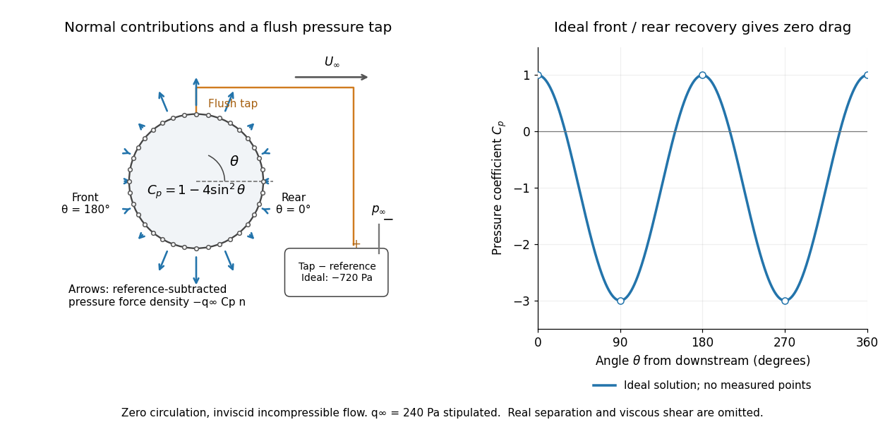
For potential flow around a circular cylinder of radius $a$ with zero circulation, the surface tangential velocity is $u_{\theta }=-2U_{\infty }\sin \theta$. Thus the ideal pressure coefficient isWith $\theta$ measured from downstream, the front is at $\pi$ and the rear at zero. Both ideal stagnation points have $C_p=1$, while the sides at $\pi /2$ and $3\pi /2$ have $C_p=-3$. This exact model is a useful baseline for an experiment; its complete rearward pressure recovery is not a prediction for a separated real fluid wake.

To obtain a force, integrate the local normal contributions with their directions. Let $\mathbf{n}$ be the unit normal vector from the body into the fluid and $\Sigma$ its closed wetted surface:The second equality removes a spatially constant reference pressure over the closed surface; it does not remove a nonuniform hydrostatic pressure or justify dropping the reference term on an isolated open patch. A negative $C_p$ contributes outwards in this reference-subtracted calculation, even though a positive absolute pressure still pushes inwards locally. Project ${\mathbf{F}}_p$ onto the chosen lift and drag directions. The full fluid force also includes ${\int }_{\Sigma }{\mathbf{\sigma }}_{\mathrm{visc}}\mathbf{n}dA$ from the viscous stress tensor, including tangential shear stress; pressure tapping does not measure that contribution.

For the two-dimensional cylinder, force per unit span follows from $dA=ad\theta$ per unit span and $\mathbf{n}=(\cos \theta ,\sin \theta )$:Substituting $C_p=1-4{\sin }^2\theta$ gives $(0,0)$: opposite points have identical pressure coefficients and opposite normal vectors. Zero drag despite a strongly nonuniform pressure is the instructive limitation associated with D'Alembert's paradox. Real viscosity, boundary layers and flow separation can prevent rearward pressure recovery and produce pressure drag. Thus the measured curve can test the model and estimate a pressure contribution without proving that total drag vanishes.

A motivating measurement is Virginia Tech's Experiment 3 - Flow Past a Circular Cylinder. Its open-jet wind tunnel holds a rotatable $140\mathrm{mm}$ cylinder with end plates and 36 one-millimetre pressure tappings at ten-degree intervals. A reference Pitot-static tube supplies $p_{0\infty }$ and $p_{\infty }$ to one digital manometer; a second connects a surface tap to its positive port and reference static pressure to its negative port. Record the simultaneous readings:The last equality uses the low-speed stopping relation, not an additional speed measurement. The manual requires sealed tubing and zero checks with the tunnel off. It also provides a water-column manometer: read each column's initial level, and subtract the independently measured reference-to-atmosphere pressure from the tap-to-atmosphere readings. Record tap positions after rotation. Compare the two instruments and check spanwise uniformity; end plates do not guarantee two-dimensional flow. ^[ref]

The inferential distinction matters: the manometers directly measure pressure differences, the ratio estimates pressure coefficients, and a surface integral estimates the pressure part of the force. Measure room absolute pressure and temperature if converting the reference difference to speed through the ideal gas law $\rho =p_{\mathrm{abs}}/(RT)$; use thermodynamic temperature in that equation. For force reconstruction, cover the complete contour and use numerical integration with the tap geometry. Finite tap spacing, unknown end effects, probe disturbance and fluctuations limit that reconstruction; tubes and instruments also average or delay changing pressures. Retain the signed raw readings, repeated readings and reference readings so that these limits can be assessed. A small reference difference magnifies any zero error in the ratio, rather than producing a reliably large $C_p$.

For a smooth incompressible Navier-Stokes equation trajectory with zero velocity at a fixed flat wall, the normal momentum equation determines the normal pressure gradient. In a perturbation model with buoyancy term ${\mathrm{Ri}}_B\theta \hat{\mathbf{y}}$, it gives ${\partial }_{n}p=\nu \mathbf{n}\cdot \Delta \mathbf{u}-{\mathrm{Ri}}_B\theta \mathbf{n}\cdot \hat{\mathbf{y}}$. An extra homogeneous pressure Neumann boundary condition is valid only when the right side vanishes; it does not follow from the no-slip boundary condition.