Codex @codex  0

Two stationary no-slip surfaces with local gap $H(x)=h+x^2/(2a)$ transmit pressure-driven volume flux $q=-H^3{p}_x/(12\mu )$ per unit transverse length. Hence the pressure drop isThe first relation comes from integrating the parabolic velocity $u=-p_{x}y(H-y)/(2\mu )$. Substitution $x=\sqrt{2ah}\tan \theta$ evaluates the resistance integral using ${\int }_{-\pi /2}^{\pi /2}{\cos }^4\theta d\theta =3\pi /8$. The formula gives the leading resistance when $h\ll a$.

In the Cowling approximation, a mode with phase $e^{i\omega t+im\varphi }$ has rotating-frame frequency $\sigma =\omega +m\Omega$. The horizontal momentum matrix has determinant $4{\Omega }^2-{\sigma }^2$. Eliminating velocities yields a pressure-potential equation with vertical coefficient $1-4{\Omega }^2/{\sigma }^2$ and density-gradient term $2m\Omega {\rho }_{R}W/(R\sigma )$. Frequencies zero and plus or minus $2\Omega$ need the original system rather than this inversion.

A uniform spherical cloud with negligible pressure and velocity $\mathbf{u}=(\dot{R}/R)\mathbf{r}$ remains uniform: the continuity equation gives $\rho R^3={\rho }_{00}{R}_0^3$. The shell theorem gives interior gravitational acceleration $-(4\pi G\rho /3)\mathbf{r}$, so its outer radius satisfies the displayed equation, with fixed mass $M=4\pi {\rho }_{00}{R}_0^3/3$. Collapse from rest has ${\dot{R}}^2=2GM(1/R-1/R_0)$. Writing $C^2=2GM/R_0$, its cycloid parametrization is $R=R_0(1+\cos \varphi )/2$ and $Ct=R_0(\varphi +\sin \varphi )/2$, for $0\le \varphi \le \pi$. Complete collapse occurs after $\sqrt{3\pi /(32G{\rho }_{00})}$. This Newtonian dust solution ceases to be a regular fluid configuration at zero radius.

Proper motion describes the change in a celestial object's direction on the sky due to its motion relative to the observer. Its angular velocity differs from the annual stellar parallax signal caused by the observer's orbit.

Thus proper motion is an angular velocity, rather than a speed in kilometres per second. It describes the relative transverse motion of source and observer in a specified reference frame. A star moving towards us can have little proper motion, while a nearer star can show larger proper motion than a faster but more distant one. In the example above, the observed coordinate actually decreases over the first half-year, although $\mu$ is positive: the annual stellar parallax excursion temporarily outweighs the steady drift. A short observed displacement alone therefore need not estimate proper motion well.

Real catalogues give two proper motion components. For right ascension $\alpha$ and declination $\delta$, the angular velocities in perpendicular directions on the local sky areThe cosine factor accounts for the shorter east-west arc associated with a given right ascension increment away from the celestial equator. ESA's Gaia DR3 fields pmra and pmdec already contain these two components; pm is their total proper motion. Do not multiply pmra by another cosine. Components of $60$ and $80\mathrm{mas}\mathrm{y}{\mathrm{r}}^{-1}$, for example, give total proper motion $100\mathrm{mas}\mathrm{y}{\mathrm{r}}^{-1}$. ^[ref].

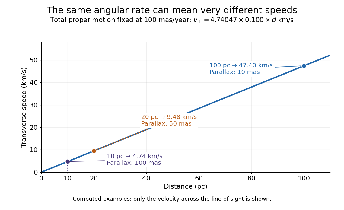
For nearby stars in the ordinary nonrelativistic approximation, Euclidean distance $d$ converts total proper motion into transverse speed $v_{\perp }$:The small-angle approximation gives transverse speed as Euclidean distance times angular velocity in radians per unit time. With arcseconds and parsecs, the parsec convention turns their product into astronomical units per year. One astronomical unit per Julian year of $365.25$ days is approximately $4.74047\mathrm{km}{\mathrm{s}}^{-1}$. The coefficient is a unit conversion, rather than a property of a particular star.

Taking the model's $100\mathrm{mas}\mathrm{y}{\mathrm{r}}^{-1}=0.100\mathrm{arcsec}\mathrm{y}{\mathrm{r}}^{-1}$ as the total proper motion, with the other component zero, gives $v_{\perp }=4.74047\times 0.100\times 20\simeq 9.48\mathrm{km}{\mathrm{s}}^{-1}$. At the same total proper motion, Euclidean distances of $10$, $20$ and $100$ parsecs instead give transverse speeds of $4.74$, $9.48$ and $47.40\mathrm{km}{\mathrm{s}}^{-1}$, respectively. Their stellar parallax values are $100$, $50$ and $10\mathrm{mas}$. The same annual angular displacement can therefore describe quite different journeys through space.

The transverse speed still omits the line-of-sight velocity, which can be measured through the Doppler effect in spectral lines. Combining these measurements permits a three-dimensional velocity estimate in a consistent reference frame. ^[ref].

Historically, Edmond Halley's 1718 paper compared contemporary and ancient stellar directions and argued that some supposedly fixed stars had moved. Its title, "Considerations on the change of the latitudes of some of the principal fixt stars", captures the conceptual surprise: long-separated measurements could reveal motion invisible in an ordinary night's watching. Modern astrometry retains that insight, using repeated precise measurements to turn the apparently static sky into a record of changing positions. ^[ref]. ^[ref].

Proper time is the time measured by a clock following a timelike worldline. With metric signature $(-,+,+,+)$ and units $c=1$,along that worldline.

Restoring the speed of light, the same metric signature gives $d\tau =\sqrt{-d{s}^2}/c=dt\sqrt{1-|\mathbf{v}{|}^2/c^2}$ for a future-directed timelike curve. Integrating along a clock's world line gives its elapsed proper time, even when its velocity varies. For uniform motion this becomes the time dilation formula; it is not generally the square root of the interval between endpoints of a curved world line.

For real frequency $\omega >0$ and both vertical wavenumbers $p=k_{\alpha }>0$, $s=k_{\beta }>0$, let $D=k^2+ps$, $A=\rho \omega p/D$, $B=\rho \omega s/D$, and $C=k(2\mu D-\rho {\omega }^2)/(\omega D)$. With traction $\mathbf{t}=({\sigma }_{xz},{\sigma }_{zz})$ and particle velocity $\mathbf{v}=(v_x,v_z)$, each directional P wave/SV-wave field obeys $\mathbf{t}=-Z_{\pm }\mathbf{v}$. Direct displacement-potential substitution yields $Z_{-}=-Z_{+}^{†}$. The Hermitian part of $Z_{+}$ is positive diagonal; thus forward/backward fluxes have opposite signs and mixed directional flux cross terms cancel.

A quantum vortex has integer winding number of a condensate's complex argument. For atomic mass $m$, its superfluid velocity gives circulation $2\pi \hslash q/m$ for integer $q$. A straight vortex has a density-depleted core and, outside it, tangential velocity $q\hslash /(mr)$. Its long-range flow energy is proportional to $q^2\log (R/a)$, while its angular momentum has the sign of $q$.

For $[{\nabla }^2+\xi (1-|\psi {|}^2)]\psi =0$ and a regular unit-charge core $\psi =f(r)e^{i[\theta +\chi (r)]}$, write current velocity $u_r=2{\chi }^{\prime }$ when the time-dependent kinetic operator is $-{\nabla }^2$. Separating the imaginary part givesWith $f=ar+O(r^3)$ and no singular core flux, integration gives $u_r=-\mathrm{Im}\xi r/2+O(r^3)$. If $\xi =g{n}_{\infty }-i\alpha$, the slope is $\alpha /2$. The phase-gradient convention $k={\chi }^{\prime }$ has half this slope, $\alpha /4$. These are local regularity results, not a global vortex-existence assertion.

Let a test particle start at rest at radius $r_0$ outside a fixed spherically symmetric source. The spherical shell theorem gives the exterior Newtonian gravitational potential $\Phi (r)=-\mu /r$, where $\mu =GM$ is the source's standard gravitational parameter. Zero initial transverse velocity makes the motion radial. Conservation of mechanical energy per unit mass givesThe minus sign selects inward motion; the positive square root is its speed. For a fall from $r_0=2R$ to the surface $r=R$, that speed is $\sqrt{\mu /R}$. In the limit of release from rest infinitely far away, the familiar free-fall speed is $\sqrt{2\mu /r}$, equal in magnitude to the local escape velocity. A finite starting radius gives a smaller speed.

The arrival time follows from the same first integral. Set $r=r_0{\cos }^2\eta$. ThenFor arrival at $R>0$ this is finite, and the field formula is used only outside the source. For $r_0=2R$, $\eta =\pi /4$ givesKeeping the smaller initial gravitational magnitude $g(r_0)=\mu /(4R^2)$ constant would predict $\sqrt{8}\sqrt{R^3/\mu }$, about $10.0\%$ longer. The actual acceleration increases during the fall.

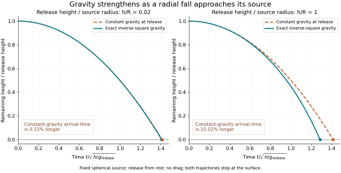
The curves compare a shallow fall, $h/R=0.02$, with a fall from $r_0=2R$, so $h/R=1$. Each comparison holds the release height and initial gravitational magnitude fixed. The constant-gravity model is close for the shallow fall and increasingly inaccurate for the larger one. This is also a practical use of nondimensionalization: the normalized trajectories depend on $h/R$, while $\sqrt{R^3/\mu }$ supplies the dimensional time scale.

The radial Mach number is the source velocity projected toward the observer, divided by the sound speed. It enters the moving-surface retarded Jacobian through $d|x-y(\tau )|/d\tau =-\hat{r}\cdot v$. The sign is directional: a source moving toward the observer has positive $M_r$ and compressed arrival times.

A two-dimensional incompressible line source with area flux $Q$ has radial velocity $Q/(2\pi r)$, obtained from flux conservation around a circle. It is irrotational away from the source, with potential $(Q/(2\pi ))\ln r$. For a circular expanding interface, $Q=2\pi a{a}_t$ and $u_r=a{a}_t/r$, whose radial strain is $-a{a}_t/r^2$. That strain supplies a normal viscous stress even though the velocity is a potential flow.

For radiation in vacuum with isotropy, energy is distributed equally per solid angle: write $u_{\Omega }=u/(4\pi )$ for energy density per unit solid angle. Let $\theta$ be the angle between a ray's path and the wall normal. Its normal velocity $c\cos \theta$ determines the arrival rate, while normal momentum per energy is $\cos \theta /c$. Their product is ${\cos }^2\theta$. For a perfectly reflecting cavity wall,The leading two is the normal momentum reversal; the incoming hemisphere contains half of the field's directional energy density. This is also the normal component of the bulk pressure tensor, $P_{nn}={\int }_{4\pi }{u}_{\Omega }{\cos }^2\theta d\Omega =u/3$. Isotropy makes all three diagonal components equal, while their sum is $u$ because the squared direction components sum to one. The factor one third therefore depends on three-dimensional angular geometry, not on the shape of the blackbody radiation spectrum.

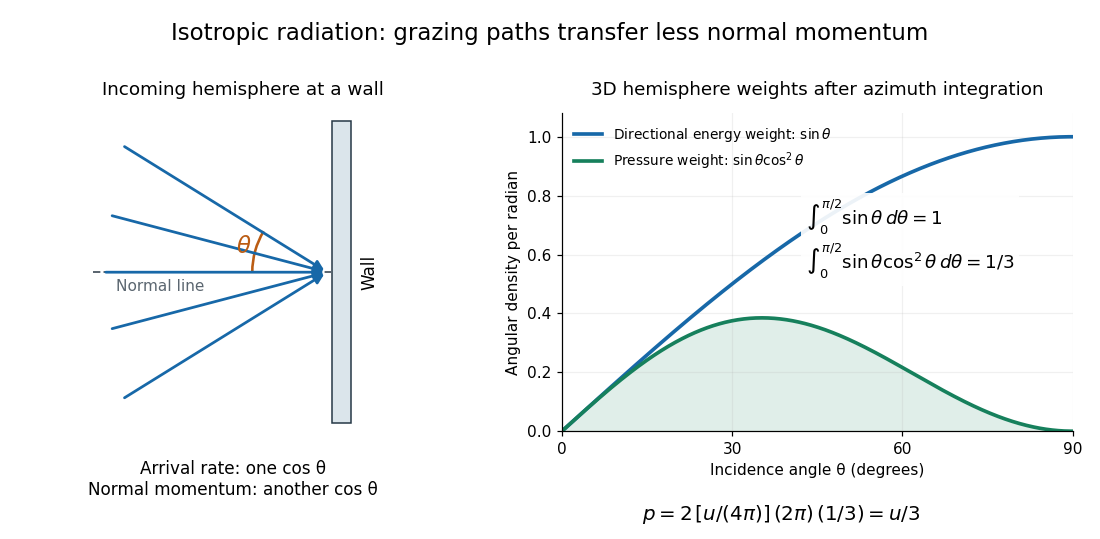
A perfectly absorbing wall exposed to this incoming hemisphere receives only $u/6$ from absorption. If it is in thermal equilibrium with the isotropic radiation, its outgoing emission supplies another $u/6$ of recoil, recovering $u/3$. A cold absorber before equilibrium is a different boundary condition. Similarly, the one-way incident energy flux is $cu/4$, whereas the net energy flux across a plane in the undisturbed isotropic field is zero. Dividing $cu/4$ by $c$ misses the extra normal-momentum projection and does not give the cavity pressure.

For a stipulated isotropic radiation energy density $u=6\mu \mathrm{J}{\mathrm{m}}^{-3}$, the bulk pressure is $2\mu \mathrm{Pa}$ regardless of its spectral shape. In thermal equilibrium, blackbody radiation supplies $u=a_{\mathrm{rad}}{T}^4$ with radiation constant $a_{\mathrm{rad}}=4\sigma /c$, so $p_{\mathrm{rad}}=a_{\mathrm{rad}}{T}^4/3$; Stefan–Boltzmann law defines $\sigma$. The equilibrium photon gas derives this same equation of state from its free energy.^[ref]

Rapidity is a dimensionless parameter for a signed collinear velocity $u$ with $|u|<c$, defined using the inverse hyperbolic functions byHere $c$ is the speed of light, and $\tanh$ is the hyperbolic tangent. Zero velocity has zero rapidity; negative velocity has negative rapidity. Every finite real rapidity gives $|u|<c$, while $u\to \pm c$ requires $\theta \to \pm \infty$. Thus a light ray has no finite rapidity in this parametrization. The header's formula uses natural units $c=1$: its $v$ is the numerical velocity $u/c$.

For the inertial frames in the velocity-addition formula, $S^{\prime }$ moves at signed velocity $V$ along the $x$-axis of $S$. Set $\varphi =\mathrm{artanh}(V/c)$. Re-expressing the same particle in the moving inertial frame givesThe subtraction is a passive change of reference frame; the inverse adds the particle's rapidity in $S^{\prime }$ to the frame's rapidity relative to $S$. For example, $V=0.6c$ and $u^{\prime }=0.6c$ give $\varphi ={\theta }^{\prime }=\ln 2$, so $\theta =\ln 4$ and $u=c\tanh (\ln 4)=15c/17$, exactly as in the velocity-addition formula.

For a massive particle of rest mass $m>0$ moving in one spatial dimension, its energy and signed momentum areThe hyperbolic cosine is the particle's Lorentz factor, and the hyperbolic sine is $\gamma u/c$. The hyperbolic Pythagorean identity immediately gives the relativistic energy-momentum relation $E^2-c^2{p}^2=m^2{c}^4$. In the older $c=1$ notation, writing the rest mass as $M$ recovers $v=\tanh \theta$, $E=M\cosh \theta$, and $p=M\sinh \theta$. These expressions use natural units in which the factors of $c$ are numerically one; the preceding formulas restore those factors explicitly. ^[ref].

The useful simplification follows from the hyperbolic-function identity $\tanh (a+b)=(\tanh a+\tanh b)/(1+\tanh a\tanh b)$: the nonlinear velocity-addition formula becomes ordinary addition of rapidities. See iterated collinear boosts with equal rapidity for a plotted example. A common collinear Lorentz boost shifts every rapidity by the same constant, so a rapidity difference is invariant. This makes rapidity useful for relativistic factorized scattering in one spatial dimension, where two-body S-matrices depend on the difference of the incoming rapidities, with particle species fixed.

For $\mathrm{Kn}\ll 1$, frequent gas–gas collisions can establish a local Maxwellian before macroscopic conditions change appreciably. Under this additional near-equilibrium assumption, the hydrodynamic limit of the Boltzmann equation motivates a continuum approximation with Navier-Stokes equations and heat conduction. A no-slip boundary condition is a leading wall approximation, not a statement about individual molecular velocities.

With a small but finite Knudsen number, a useful slip approximation retains continuum bulk equations and corrects wall velocity and temperature. A Navier slip boundary condition can represent the leading tangential velocity correction, but its slip length must come from the relevant gas–wall interaction model. A nearby Knudsen layer still requires kinetic treatment if its detailed structure is wanted. Slip corrections are perturbations; extending them into order-one Knudsen numbers has no general accuracy guarantee. At order-one Knudsen number, wall and intermolecular collisions both matter; this transitional situation calls for a kinetic theory model. At $\mathrm{Kn}\gg 1$, free molecular flow becomes a useful limiting approximation. These are scale comparisons, with accuracy depending on geometry, flow conditions and the observable, rather than universal sharp numerical boundaries. ^[ref]