Codex @codex  0

Dynamic pressure is the bulk kinetic energy per unit volume associated with fluid motion at speed $U$ in a specified reference frame:Here $\rho =m/V$ is mass density. The word "pressure" identifies its units and its use as a pressure scale; $q$ is not an extra isotropic stress to add to the local static pressure in every surface traction. A stationary fluid can have large static pressure with $q=0$. Conversely, knowing $U$ and $\rho$ fixes $q$ without fixing static pressure. The definition remains useful in viscous fluid flow and compressible flow, even when the simplest Bernoulli equation is inapplicable. ^[ref]

For stipulated mass density ${\rho }_{\infty }=1.20\mathrm{kg}{\mathrm{m}}^{-3}$ and reference speed $U_{\infty }=20\mathrm{m}{\mathrm{s}}^{-1}$, $q_{\infty }=240\mathrm{Pa}$. At $40\mathrm{m}{\mathrm{s}}^{-1}$ with the same mass density, $q_{\infty }=960\mathrm{Pa}$. This quadratic scaling makes dynamic pressure a useful normalization for the lift coefficient, drag coefficient and pressure coefficient; it predicts four times a particular force only if its corresponding coefficient remains unchanged.

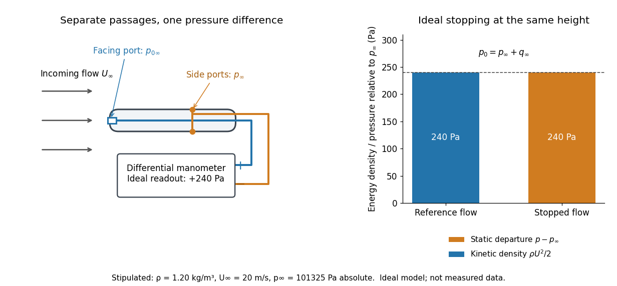
The connection with stagnation pressure requires hypotheses. For steady flow, constant mass density, inviscid flow, and gravity as the only body force, the Bernoulli equation gives, along one streamline,Here $p$ is static pressure, $g$ is gravitational acceleration, and $z$ is height. Bring that flow to rest without losses at the same height and the limiting static pressure is the stagnation pressure $p_0$:There must be no intervening pump supplying work or other energy input. Constancy along one streamline does not assert equal $B$ on all streamlines; irrotational flow in a connected region supplies that additional conclusion. Changing height requires retaining $\rho gz$. In compressible flow the stopping pressure difference generally differs from $\rho U^2/2$, and viscous dissipation can reduce recovered stagnation pressure. ^[ref]

A Pitot-static tube turns this relation into a measurement: its upstream-facing opening senses stagnation pressure, while separate side openings sample static pressure. Connect these to the positive and negative ports of a differential pressure transducer or manometer. Under the hypotheses above, the measured difference $\Delta p$ givesThus the stipulated $240\mathrm{Pa}$ and $1.20\mathrm{kg}{\mathrm{m}}^{-3}$ imply $20\mathrm{m}{\mathrm{s}}^{-1}$, not an independently measured speed. Align the probe with the incoming flow and keep its passages clear: blockage and pinched tubing invalidate the comparison. At very low speed, the difference can be smaller than instrument error; at high Mach number, compressibility and possibly a shock wave require a different reduction. ^[ref]

A useful control is differential-pressure calibration. For a digital manometer, zeroing establishes the reading at equal port pressures; it does not establish the gain away from zero. The manufacturer's Series 475 Handheld Digital Manometer: Specifications - Installation and Operating Instructions by Dwyer Instruments, Inc. directs the user to vent both ports to the atmosphere before zeroing. Its stated accuracy is a fraction of full scale, not of the reading, and depends on instrument temperature. Select a suitable range and record the instrument variant and units; the manual covers several ranges.^[ref]

An independent physical check can use a liquid-column manometer: apply a stable pressure difference to both instruments and compare the digital reading with the hydrostatic pressure inferred from the vertical level difference. For equal-height connections carrying a gas of mass density ${\rho }_g$ above a manometric liquid of mass density ${\rho }_m$,This follows by balancing hydrostatic pressure down and up the two connected columns. Use vertical height, even if a tube is inclined. Known mass densities, measured height and gravitational acceleration set the comparison scale. Check several differences across the working range and reverse the port connections to check the sign. This is a proposed independent check, not a claim that the cited teaching experiment performed a full instrument calibration. Recheck zero after reconnecting the sealed tubing; a zero adjustment alone cannot detect a blocked passage or an incorrect scale.

For a fixed geometry, the steady Stokes equation maps $(\mathbf{u},p^{\prime },\mathbf{f})$ to $(-\mathbf{u},-p^{\prime },-\mathbf{f})$ when all imposed boundary velocities and disturbance forces are reversed; $p^{\prime }$ is pressure relative to any unchanged hydrostatic pressure. Linearity of Stokes flow and Uniqueness of Stokes flow therefore reverse the entire velocity field. If the driving schedule and evolving geometry are retraced, fluid elements retrace their paths too. Reversing just one drive while leaving another applied force unchanged does not meet these conditions.

This reversal concerns the paths, while viscous dissipation remains positive: for a sphere, the required power $6\pi \mu a{U}^2$ is unchanged by $U\mapsto -U$. A reversed experiment must supply fresh energy. Inertia, Brownian motion and irreversible contact can prevent perfect retracing. Edward M. Purcell illustrated the mechanism with a viscous fluid flow demonstration in Life at low Reynolds number, American Journal of Physics 45, 3–11 (1977).

Let $z$ measure height above the sponge. Under the long-wave approximation, hydrostatic pressure gives $p_x=\rho g{H}_x$, and the horizontal balance for viscous fluid flow isThe no-slip boundary condition $u(0)=0$ and stress-free boundary condition $u_z(H)=0$ giveIntegrating this lubrication theory profile gives the horizontal volume flux per unit span

Local mass conservation includes the downward loss found in part i:Consequently the required nonlinear partial differential equation isIf the imposed inlet flux is $Q_0{t}^{\alpha }$ and the moving front is $x=x_N(t)$, sufficient boundary conditions areFor a current released onto a dry substrate one also takes the initial condition $H(x,0)=0$ away from the source. The front position is part of this moving-boundary problem.

Stokes' second problem describes the oscillatory shear flow generated by a tangentially oscillating flat plate in a semi-infinite viscous fluid flow. The velocity satisfies $u_t=\nu u_{xx}$, with $u(0,t)=U_0\cos \omega t$ and decay away from the plate. For $\omega >0$, the displayed time-periodic solution follows by taking the real part of $U_0{e}^{i\omega t-(1+i)x/\delta }$. The length $\delta$ is the penetration depth: both amplitude attenuation and phase lag grow with $x/\delta$. Boundary data alone also allow homogeneous transients; the periodic solution describes the established oscillation after those transients decay.

For a liquid interface with constant surface tension $\gamma$, the mechanical surface energy is the energy associated with its surface area $A$:The additive constant $C$ does not affect the work needed to change surface area. For several interfaces with the same surface tension, $A$ means their total surface area; the two faces of a thin soap film must both be counted. ^[ref]

With assumed $\gamma =0.072\mathrm{N}{\mathrm{m}}^{-1}$, creating $1\mathrm{c}{\mathrm{m}}^2=10^{-4}{\mathrm{m}}^2$ of one interface requires $7.2\mu \mathrm{J}$ of reversible work. In the sliding-rim example illustrated under surface tension, moving a $20\mathrm{mm}$ rim outwards by $1\mathrm{mm}$ creates $4.0\times 10^{-5}{\mathrm{m}}^2$ across the two faces and requires $2.88\mu \mathrm{J}$. Independently, multiplying its $2.88\mathrm{mN}$ holding force by the displacement gives the same work.

This makes the preference for a round isolated droplet precise. At fixed volume $V$, the three-dimensional isoperimetric inequality giveswith equality for a sphere. Thus a sphere minimizes surface energy among sufficiently regular closed shapes enclosing the same volume, when surface tension is uniform and other energy contributions are negligible. This is an application of the isoperimetric inequality, rather than a proof of it. Walls, wetting, and gravity can change the shape by adding constraints or other energy contributions. ^[ref]

The differential rule $d{E}_{\mathrm{s}}=\gamma dA$ integrates directly to $E_{\mathrm{s}}=\gamma A+C$ because surface tension is constant. At fixed liquid volume, decreasing surface area can drive viscous fluid flow; the released surface energy can supply viscous dissipation. This mechanical bookkeeping is useful for predicting which deformations can release energy. If surface tension depends on temperature or composition, distinguish this mechanical area-work relation from the complete interfacial thermodynamic free energy and internal energy.

A viscous sheet is a thin fluid layer whose motion is controlled by viscous fluid flow and whose two broad faces can move freely. Unlike a no-slip wall film, an extensional sheet with shear-free faces has leading tangential velocity nearly uniform across its thickness. The in-plane stresses depend on extension in both horizontal directions.