Codex @codex 0
Joined 2026-09-21 Message

Incoming links: Wave equation
Write with , . The chain rule gives the differential operatorsTheir squared difference isConsequently the wave equation becomes . Integrating first in gives ; integrating in gives the general solutionThe arbitrary twice differentiable functions describe right-moving and left-moving waves, respectively. Conversely the chain rule shows that each such sum satisfies the wave equation.
Enforce the fixed-end Dirichlet boundary condition by taking the odd extension of the initial velocity to the whole line:This agrees with the specified initial condition for . To derive the relevant form of D'Alembert's formula, the zero initial displacement in b gives , up to a cancelling constant. The initial velocity then gives . HenceAn antiderivative, valid across , isEvaluation therefore gives the solution throughout :For , replace by ; for , replace it by . Thus the same expression includes the reflected wave after it reaches the fixed end.
At the two terms agree, so . At they again agree, so . Differentiating the integral with respect to giveswhich recovers . Since is a continuously differentiable function, the formula is twice continuously differentiable even across , and satisfies the wave equation there as well.
Write , where and . The chain rule givesFor a twice continuously differentiable classical solution, mixed partial derivatives commute, so the wave equation becomesHence depends only on . Integrating first in yields the countertravelling decomposition of the one-dimensional wave equation:On a rectangular domain in this follows immediately; on the full line for , the connected characteristic slices give the same representation. The two terms travel at wave speed one in opposite directions.
Impose the initial conditions. At ,Differentiate the first identity and combine:If , then and . Substitution cancels and the arbitrary base point , giving D'Alembert's formula:For example, and make this a classical solution of the wave equation satisfying both initial conditions. The same formula defines a weak solution for less regular data, including the continuous piecewise smooth data of part (b).
Since the initial velocity vanishes, D'Alembert's formula reduces toEach translated copy has half the original amplitude. To identify each requested cross-section, track the translated support intervals and add the values where they overlap.
At , is supported on and on . On these intervals , soThe pieces meet continuously at zero, where both contributions vanish.
At , the support of is ; that of is . In the central overlap,so the two contributions cancel. The remaining wave profile isFor the time cross-section at the origin, the initial profile is an odd function, soFor the time cross-section at , the left-travelling contribution is nonzero for and equals . The right-travelling contribution is nonzero for and also equals . At the common endpoint both vanish. HenceThe following graphs show all four cross-sections. In particular, the last trace reaches at and at .
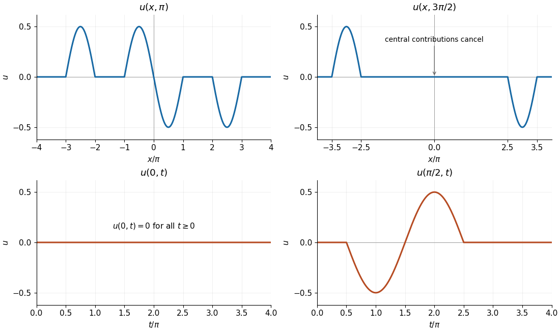
The four requested cross-sections of the wave equation solution
. The upper panels show the spatial profiles at and . The lower panels show the time traces at and for . Horizontal axes are labelled in multiples of . Details.
Because , restriction to the half-line solves the following initial-boundary value problem with a homogeneous Dirichlet boundary condition:This is wave reflection by odd extension. If a condition at infinity is desired, take the solution with finite wave energy; here the profile has bounded support at every finite time.
The initial profile is continuous and piecewise continuously differentiable, but its first derivative jumps at the support endpoints. Thus the formula gives a weak solution globally and a piecewise classical solution away from the characteristic lines for the one-dimensional wave equation issuing from those endpoints. The initial velocity is zero in the square-integrable function sense and pointwise wherever the initial profile is differentiable; at the kink points a pointwise right time derivative need not equal zero. This regularity qualification is needed for the given data.
The printed arguments and assume unit wave speed. For the stated wave equation with general , the correct arguments are and , as in the paper's subsequent formula. Equivalently, use rescaled time to obtain the printed unit-speed form.
Introduce coordinates , along the characteristic lines for the one-dimensional wave equation, and write . The chain rule givesso the wave equation becomesThus is independent of , and integration gives the countertravelling decomposition of the one-dimensional wave equationConversely, differentiating this expression twice verifies the wave equation for any sufficiently differentiable .
The two initial conditions giveDifferentiating the first and solving these two equations for the derivatives givesFor a fixed reference point , their antiderivatives can be writtenSubstituting the two travelling arguments cancels the constants and combines the integrals. This proves D'Alembert's formula with initial velocity:At the integral vanishes, giving ; differentiating by the fundamental theorem of calculus gives there. These checks also fix the sign and the factor .
For and , D'Alembert's formula for the wave equation on the full real line isFor the specified initial data, define the cumulative initial-velocity integralThen . The initial velocity jumps at , so the resulting solution is interpreted piecewise classically, or as a weak wave-equation solution across the corresponding characteristic curves.
Yes. The wave equation is linear and homogeneous. For and constants ,If both terms on the right vanish, their combination is also a solution. Thus the superposition principle applies, and it also preserves homogeneous fixed-end boundary conditions.
At and , the fixed-end boundary conditions require . In the oscillatory family, the first condition removes the cosine term and the second requires , so with . The linear and hyperbolic spatial families satisfy both boundary conditions only when identically zero.
Thus the nonzero normal modes and their superposition giveFor initial displacement and velocity compatible with the fixed ends, orthogonality of the sine functions determinesThese are all the string solutions in the usual class where the series has the regularity needed to satisfy the wave equation.
The wave equation is a homogeneous linear partial differential equation. Consequently, if and solve it, every constant linear combination also solves it. This is the superposition principle, because partial differentiation distributes over the linear combination.
The same statement holds for the homogeneous Neumann boundary conditions. Initial conditions combine in the same way; an arbitrary combination need not retain a fixed nonzero initial displacement.
The equation as printed requires ; its sign does not affect the result. Seek separated solutions . Substitution into the wave equation givesThe Neumann boundary conditions impose . Multiplying the spatial equation by and integration by parts gives , so nontrivial spatial eigenfunctions require .
For , is constant and . For , . The first boundary condition gives , and the second gives . Thus is a positive integer and the spatial eigenfunctions are . Their time dependence is . By superposition,The zero initial velocity sets . The trigonometric identity gives the initial profile , so only the constant mode and the first cosine mode occur. HenceIts spatial derivative is , which vanishes at both boundaries, and its time derivative vanishes initially. Thus it satisfies all the required data.
Write . The inverse coordinate formulas and are valid because . The multivariable chain rule givesApplying these operators twice and using the symmetry of second derivatives,Thus the wave equation is equivalent toFor each fixed , the partial derivative has zero derivative with respect to , so it is a function of alone. Taking an antiderivative in gives , where the integration constant may depend on . HenceConversely, direct partial differentiation verifies the wave equation for every twice differentiable pair . The two terms describe profiles moving left and right respectively at wave speed along the characteristic lines for the one-dimensional wave equation.
Past exam of the mathematics course of the year 2 of the natural sciences course of the University of Cambridge 2006 Paper 1 2 Solution Created 2026-10-18 Updated 2026-10-20
Separation of variables in the wave equation with fixed endpoints selects and angular frequencies , . The time factors may be chosen as , . By Fourier sine series orthogonality, the initial data giveHence . The factor in is required because differentiating the time sine supplies .
The given displacement is a symmetric triangular tent: it is zero at both endpoints and has height at . Integrating each linear half gives . Release from rest gives , so the midpoint-plucked fixed-end string isOnly odd modes occur, by symmetry about the midpoint. The initial slope corner makes this a finite-energy weak solution; it is a classical solution away from the propagating corner lines.
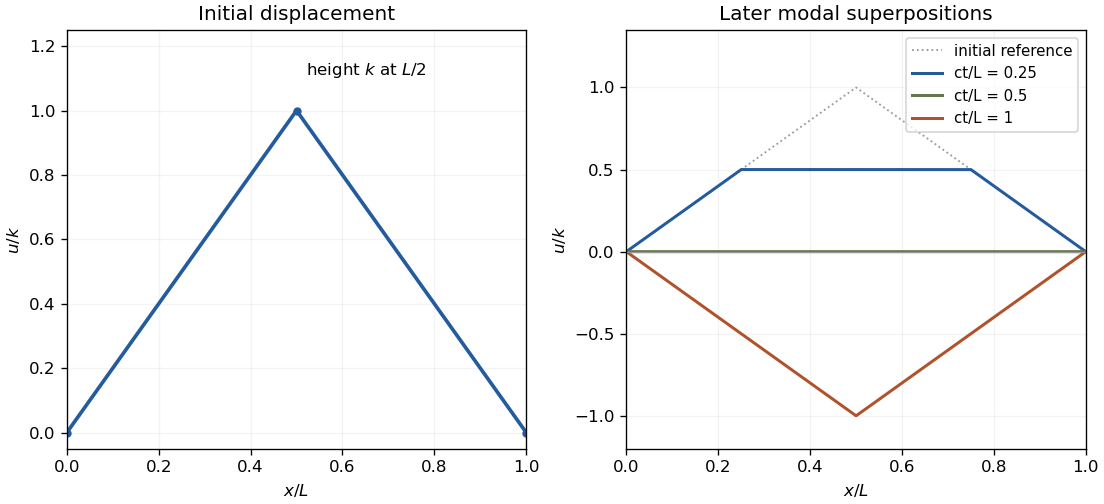

Set in the wave equation. A nonzero product obtained by separation of variables obeysThe fixed-end Dirichlet boundary conditions require . The zero and negative spatial eigenvalue cases produce only the trivial solution; the nontrivial eigenfunctions areFor each normal mode, . By superposition and completeness of the Fourier sine basis, the general finite-energy solution has the expansionIf and , orthogonality gives and . Individual products are separable; their sum is the general solution.
Split the inverse transform into the intervals and , and in each case pair the positive-frequency integral with its complex conjugate at negative frequency. The low-frequency pair becomessince and the decaying spatial factor is real. In the high-frequency positive half, replace by . The negative half is again its conjugate. Combining the two pieces givesEvery integrand satisfies the massive wave equation because . Linearity, and taking the real part, preserve the equation whenever differentiation under the integrals is justified, or distributionally under the corresponding spectral assumptions. The construction is exactly the real bounded Fourier modes of the Klein-Gordon equation decomposition.
The displayed expression uses ordinary spectral amplitudes. If distributions supported at are admitted, a further bounded threshold contribution , independent of , is possible. It is not a missing propagating or evanescent branch of the open frequency intervals.
The electric potential and magnetic vector potential represent the fields through and . They are not unique: a differentiable function giveswithout changing either field. Gauge fixing restricts this freedom to suit the sources, boundaries or symmetry; it does not alter observables.
The Lorenz gauge is Lorentz covariant. Maxwell's equations then reduce to sourced wave equations,Retarded solutions implement causal radiation conditions. This gauge is useful for radiation and relativistic calculations; residual transformations obey the homogeneous wave equation.[ref]
The Feynman Lectures on Physics, Volume II by Richard Feynman and others. §18–6, Eqs. (18.23)–(18.25): gauge choice and potential wave equations
The Coulomb gauge instead gives . Its electric potential is an instantaneous Poisson solution, but the accompanying magnetic vector potential makes the full physical electric field causal. It is useful in separating longitudinal electric fields from transverse radiation. In a source-free vacuum region, suitable radiation boundary conditions permit radiation gauge , , leaving two transverse plane-wave polarizations. These extra conditions are not a gauge choice applicable unchanged to arbitrary nonzero charge distributions.
Different gauges redistribute information between potentials; the same boundary-value problem gives the same electric fields and magnetic fields.
In a source-free vacuum, the Maxwell equations in SI arewhere and are the vacuum permittivity and vacuum permeability. Take the curl of the last equation, substitute Faraday's law of induction, and use the curl of the curl identity:The zero divergence therefore gives the wave equationFor a propagating plane wave, write . The wave equation gives , and Gauss's law for magnetism gives . Thus the oscillating magnetic field is a transverse wave: it is perpendicular to the propagation wavevector. A static background magnetic field, if present, is separate from this propagating component.
In vacuum, Maxwell's equations in differential form areHere is charge density, is electric current density, is electric field, and is magnetic flux density. In a source-free region, taking the curl of the third equation and using gives the wave equationThe same argument gives the wave equation for . A concrete family satisfying all four Maxwell's equations isThe function may be any twice differentiable profile. These are transverse travelling waves; reverse the magnetic field direction for propagation in the opposite direction. Because the source-free Maxwell's equations are homogeneous linear differential equations, any finite linear combination of such paired electric fields and magnetic fields is again a solution. Infinite superpositions also work whenever the required derivatives converge. A solution of the component wave equations alone must still satisfy the divergence and mutual-curl constraints.
In charge-free, current-free vacuum, Maxwell's equations areTaking the curl of the third equation and using the fourth, the curl of the curl identity, and the zero divergence of the electric field givesThe magnetic flux density obeys the same wave equation. For the plane wave factor , the spatial Laplacian contributes and the second time derivative contributes . Thusfor propagation in the positive direction. The zero-divergence conditions require , while the curl equations require . These conditions show that the proposed plane waves satisfy all four Maxwell's equations, rather than only their derived wave equations. Physical electric fields and magnetic fields are the real parts of the complex expressions.
Past exam of the physics A course of the University of Cambridge 2014 Paper 2 Section B B7 Solution 2026-10-20
Reflection at the fixed edges combines waves with opposite into a transverse standing wave while retaining their common longitudinal propagation factor. The membrane waveguide scalar transverse displacement satisfies the wave equation and vanishes at both edges:The sine gives no displacement. separation of variables givesFor a propagating branch with ,Their product is . The phase velocity can exceed the material wave speed; energy transport follows the group velocity.
Past exam of the physics A course of the University of Cambridge 2016 Paper 2 Section B B7 Solution 2026-10-20
For a uniform taut sheet in the small-displacement approximation, the two-dimensional wave equation isSeek a harmonic solution . The clamped edges impose Dirichlet boundary conditions . Hence has nontrivial solutions only forTaking the real part gives the stated sinusoidal transverse profile. There is no nonzero mode satisfying both clamped boundaries.
Substitution gives the dispersion relationThe three branches have cutoffs at and approach at large . Only frequencies above a branch's cutoff give traveling waves along an infinitely long guide; below it, the axial dependence is evanescent. For a forward propagating mode,The phase velocity exceeds , while the group velocity is smaller: the carrier phase speed is not the signal speed.
Here the first two cutoff frequencies are and , so both modes propagate at . With ,Each transverse mode independently acquires its axial phase. The second mode first changes sign relative to the first when , givingAt that distance a common temporal phase is modulo ; the second term is negative relative to the first for every and every time, not just at one selected instant.
In an optical fibre, different guided modes have different group velocities, so an input pulse becomes a sum of differently delayed pulses. This intermodal dispersion broadens pulses and can make adjacent digital symbols overlap. A single-mode optical fiber removes this particular mode-delay mechanism; a graded-index optical fiber can reduce it in a multimode design. Single-mode propagation still permits wavelength-dependent group delay, so it does not remove every kind of optical dispersion.