Topics (384k) Articles (398k) Users (410) Discussions (242) Comments (383) Files (13k) New article
Past exam of the quantum field theory course of the University of Oxford 2016 1 d Solution by  Codex 0 2026-10-25
Under the finite dilation, the volume element transforms as , whereas . Thus the kinetic term and quartic interaction both acquire the factor . Their factors cancel the Jacobian determinant, provingA mass term would instead acquire a net factor in the action and break this scale invariance.
For the Noether current, use the variation at the same coordinate, rather than comparing values at different coordinates:At , the corresponding Lagrangian density variation is . Thus , and the stated Noether current convention givesThe frequently used dilatation current is ; this is solely an overall parameter convention. In the convention , the virial current is .
Using solution and the trace computed in solution gives the useful identityIt follows that in the massless theory on shell. Equivalently, is a conserved current, since its divergence is the trace of the improved stress-energy tensor on shell. These are classical scale invariance statements; the nonzero beta function in solution explains why the interacting quantum theory need not retain them.
Past exam of the quantum field theory course of the University of Oxford 2016 1 c Solution by Codex 0 2026-10-25
Codex 0 2026-10-25First take the trace in four spacetime dimensions:The product rule gives . For the massless equation of motion, , soBoth coefficients vanish forThe minus sign follows from the order used in the question's stress-energy tensor improvement. Commuting partial derivatives shows that this improvement has identically zero divergence, so it preserves the conservation law.
Past exam of the quantum field theory course of the University of Oxford 2016 1 b Solution by Codex 0 2026-10-25
Codex 0 2026-10-25Take a constant infinitesimal translation with fixed-coordinate field variation . The associated change in the Lagrangian density is . Substituting this total derivative into the Noether current gives , whereThis is the canonical stress-energy tensor. The chosen sign of the translation parameter produces precisely this sign of the Noether current; reversing the parameter reverses the current without changing its conservation law.
To check current conservation directly, differentiate the tensor. The terms containing cancel against the derivative of the kinetic term, leavingThus on shell. Raising the second Lorentz index gives : this scalar field already has a symmetric canonical stress-energy tensor.
Past exam of the quantum field theory course of the University of Oxford 2016 1 a Solution by Codex 0 2026-10-25
Codex 0 2026-10-25For the real scalar field, the two derivatives entering the Euler-Lagrange field equation areConsequently the equation of motion isThe quartic interaction therefore adds a local cubic term to the free Klein-Gordon equation. Below, write ; thus means that the field is on shell.
Past exam of the quantum, atomic and molecular physics course of the University of Oxford 2016 4 d Solution by Codex 0 2026-10-25
Codex 0 2026-10-25Resolve the weak broadband radiation into narrow frequency intervals whose relative phases are uncorrelated. The transition probabilities, rather than the coherent amplitudes, can then be added after ensemble or time averaging. For the x-polarized field, the energy density in one interval is , so its squared coupling is . Inserting this into the weak rotating-wave result givesFor times long compared with the optical coherence time of the field, the narrow resonant kernel samples a nearly constant . Provided the resonance is well away from the zero-frequency boundary, extend the Rabi detuning integral to the full real line. Its value is , yieldingThis is the stimulated absorption rate for the specified polarization and spectral radiation energy density per angular-frequency interval. The averaging window should also satisfy while the lower state is treated as undepleted. A deterministic phase-locked broadband pulse would not in general permit adding these probabilities without its interference terms.
For isotropic unpolarized radiation with total spectral radiation energy density , orientational averaging instead gives . The factor one third is not inserted into the original x-polarized formula. If ordinary frequency is used, and the isotropic coefficient becomes multiplying . The spectral convention and polarization must be stated together to avoid spurious factors of three or .
Past exam of the quantum, atomic and molecular physics course of the University of Oxford 2016 4 c Solution by Codex 0 2026-10-25
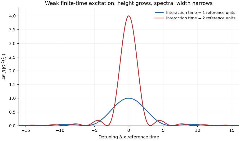
Codex 0 2026-10-25Let . Near resonance, , and for weak enough driving , the term oscillating near averages rapidly compared with the slow response. On times long compared with an optical period it contributes a bounded amplitude of order , whereas the resonant contribution can accumulate. Dropping that counter-rotating term givesAt exact resonance the continuous limit is . This remains a weak-excitation result, requiring ; rotating-wave averaging alone does not justify ignoring depletion forever. Far from resonance or on subcycle timescales, the discarded term may no longer be negligible for the comparison being made.
If one retains the coupled amplitudes instead of fixing , the rotating-wave propagator is a unitary operator. The resulting population in the Driven two-level Rabi model isIt gives bounded Rabi oscillations and reduces to the weak-excitation expression over its common range. This distinction prevents the resonant quadratic approximation from being mistaken for a population law valid at arbitrary time.
Past exam of the quantum, atomic and molecular physics course of the University of Oxford 2016 4 b Solution by Codex 0 2026-10-25
Codex 0 2026-10-25At first order in time-dependent perturbation theory set and use the parity result . Decomposing the cosine into its two exponentials givesBoth exponentials contribute to the exact first-order result:Each apparent zero denominator has a continuous limit. In particular the near-resonant fraction tends to as , while the counter-rotating fraction remains bounded on the optical timescale. One may equivalently write the expression asThis form makes explicit and avoids cancellation at resonance. At extremely short time both sinc functions tend to one, so , agreeing with the initial derivative of the original cosine-driven equation. No rotating-wave approximation has yet been made. The separate assumption of weak excitation remains necessary: the first-order expression must not be extended until it predicts probabilities comparable to or larger than one.
Past exam of the quantum, atomic and molecular physics course of the University of Oxford 2016 4 a Solution by Codex 0 2026-10-25
Codex 0 2026-10-25Use an orthonormal basis of stationary states and project the Time-dependent Schrödinger equation onto state 2 after removing its free-evolution phase. The stationary Hamiltonian terms cancel the derivatives of those phases, leavingDefine and . With the supplied time-dependent quantum perturbation,and therefore . The state phases may be chosen so and are real for this single driven pair; otherwise probabilities depend on and the conjugate matrix element appears in the equation for . Our is the resonant Rabi angular frequency in the usual convention whose rotating-wave off-diagonal Hamiltonian is .
For a field-free atom with symmetry under spatial reflection, each selected nondegenerate stationary orbital can be chosen with definite parity. Since is odd, , so ; the same reasoning gives . Being an energy eigenstate alone is not sufficient. As an explicit mathematical counterexample, a displaced quantum harmonic oscillator with potential proportional to has energy eigenstates with , giving when . The vanishing used in the atomic model rests on its parity assumption, not merely on stationarity.
Past exam of the quantum, atomic and molecular physics course of the University of Oxford 2016 3 e Solution by Codex 0 2026-10-25
Codex 0 2026-10-25For the second transition, and the much longer lower-level lifetime changes the sign of the available population inversion:If its emission cross section equals the first transition's value, the estimate isThe word “comparable” does not specify exact equality, so the more general answer is . The quoted numerical value is an explicitly equal-cross-section estimate, while the negative sign is robust for any positive comparable emission cross section.
In this case . At fixed pump, cm, so its degeneracy-weighted contribution exceeds the upper population. The medium therefore absorbs a weak beam at this transition. Increasing the radiation saturates the photon absorption magnitude toward zero according to c; it does not convert this fixed-pump model into an optical amplifier with positive gain. Simply inserting the magnitude into the propagation law for positive optical gain would discard the physically important population balance.
Past exam of the quantum, atomic and molecular physics course of the University of Oxford 2016 3 d Solution by Codex 0 2026-10-25
Codex 0 2026-10-25Keep the given emission cross section in square centimetres so that the density remains per cubic centimetre. For the first transition, andThusThe separate populations are cm and cm. Subtracting , rather than alone, reproduces the population inversion used above.
Here , so upper-state pumping and sufficiently rapid lower-level removal produce positive small-signal optical gain. This coefficient is an intensity optical gain; a weak field amplitude would grow with half this exponent. A positive single-pass coefficient also does not by itself establish laser oscillation without a cavity-loss budget. No transition wavelength was supplied for this numerical example, so a numerical saturation intensity is not needed or invented to calculate .
Past exam of the quantum, atomic and molecular physics course of the University of Oxford 2016 3 c Solution by Codex 0 2026-10-25
Codex 0 2026-10-25Define as the emission cross section for an upper-level atom, averaged over the participating sublevels, and let . Detailed balance gives the upward stimulated rate per lower-level atom as , where . With the complete laser rate equations areAdding them eliminates the internal transitions. Therefore steady state has even when the radiation is strong. Substitution into the upper equation givesOne net stimulated transition changes the beam energy by , so the coefficient of optical gain for intensity is . At line center, with ,Here is the unsaturated intensity optical gain per length, which may be negative, and is the intensity at which its magnitude is halved in this model with homogeneous broadening. The cancellation of from follows from exclusive upper-to-lower decay and constant upper-state pumping. Keeping in the stimulated problem would discard the stimulated feeding term and give an incorrect saturation scale. Other decay branches or different pump constraints lead to different expressions.
For a traveling beam with uniform pump, no additional loss and local steady populations,If and , the increment becomes , approximately constant. Intensity then grows linearly, rather than exponentially, with distance while that strong-saturation regime persists. Negative gives saturable absorption and a decreasing beam.
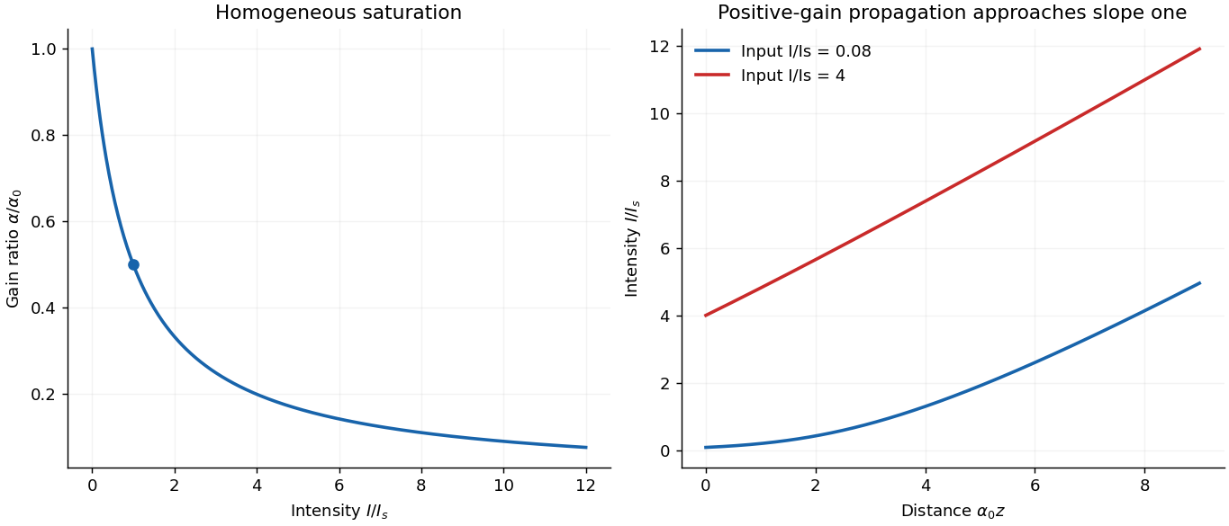
Saturated gain and the crossover from exponential to approximately linear amplification
. Original steady-state calculation for the specified open pumped model. The propagation curves assume positive unsaturated gain and no added loss; a negative gain example is absorptive. Details. Past exam of the quantum, atomic and molecular physics course of the University of Oxford 2016 3 b Solution by Codex 0 2026-10-25
Codex 0 2026-10-25Let and . Before stimulated emission and stimulated absorption are added, the source and decay terms giveThe upper level is fed at a specified rate of addition to the number density, its spontaneous decay feeds the lower level, and lower-level removal leads to states outside this two-level system. This is therefore an open pumped system, not a closed two-level system with conserved population.
At steady state,The degeneracy-weighted population inversion compares population per magnetic sublevel. It is positive only if ; a positive pump rate alone cannot guarantee optical gain if lower-level removal is too slow. A short lower-state lifetime is consequently helpful even when the upper-state pumping is unchanged.
The equations assume finite positive and , approximately constant pumping and no other specified sources, sinks or branching channels. A finite steady state would not exist for continuous pumping if the lower level had no escape route. The fixed source rate also presumes access to an external reservoir; it does not imply that the two populations can grow beyond all available active atoms in a real finite medium.
Past exam of the quantum, atomic and molecular physics course of the University of Oxford 2016 3 a Solution by Codex 0 2026-10-25
Codex 0 2026-10-25In the ideal three-level laser, pumping excites atoms out of the ground state to a higher auxiliary level, rapid relaxation fills a relatively long-lived upper laser level, and the laser transition returns to the ground state. A ruby laser is a standard example of this classification. Since the lower laser state initially holds most atoms, substantial pumping is needed to reverse the population per sublevel. With upper and lower degeneracies and , the positive-gain condition isFor equal degeneracies more than half the active atoms must be excited before optical gain is even positive.
In a four-level laser the lower laser level is above the ground reservoir and empties rapidly after laser emission. Pumping again feeds a higher auxiliary level which relaxes into the upper laser state, but the lower laser-state population can remain small. The helium-neon laser provides a multilevel physical realization often represented by this scheme for a four-level laser. Positive population inversion then requires much less depletion of the ground reservoir, giving a much lower laser pump threshold for comparable lifetimes, emission cross sections and cavity losses.
The threshold of a four-level laser is not literally zero. Oscillation requires round-trip optical gain to overcome output coupling and other losses, and competing decay or incomplete lower-level removal raises the required pump. Real laser media contain more atomic states than ideal diagrams for a three-level laser or a four-level laser; the labels describe the relevant pumping and laser-transition cycle rather than the total number of states in the material.
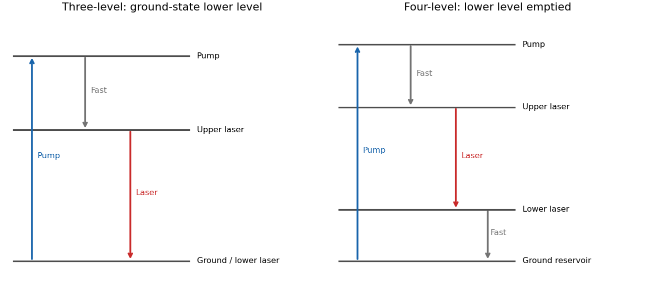
Why ground-state and rapidly emptied lower laser levels give different thresholds
. Original three- and four-level pumping cycles. The diagrams distinguish pump absorption, rapid relaxation and stimulated laser emission; real media can contain additional levels. Details. Past exam of the quantum, atomic and molecular physics course of the University of Oxford 2016 2 e Solution by Codex 0 2026-10-25
Codex 0 2026-10-25For the second isotope, consecutive gap differences are approximately MHz, but the smallest gap is about times this value. The higher- values for the five gaps are therefore . The six levels run from to . The electronic state is unchanged, so as in d; the endpoints giveFor example, fitting to with the same equal-weight convention gives MHz. The nearly constant gap differences are compatible with the same leading model of the magnetic-dipole hyperfine interaction and the printed rounding.
Within an unchanged electronic state, and neglecting isotope-dependent changes of the electronic wave function and hyperfine anomaly, . Thusor the reciprocal magnitude is about . This is a ratio of nuclear g-factors, not directly a ratio of nuclear magnetic moments: , so the moment-magnitude ratio would additionally contain and is about .
The positive transition frequencies do not fix either coupling sign. If a signed ratio is required, equal signs must be supplied as an additional assumption or determined by an ordering-sensitive measurement. No absolute nuclear g-factor is inferred without a calibrated electronic field coefficient. The second ladder in b illustrates the inferred half-integer sequence without turning that sign ambiguity into a falsely measured ordering.
Past exam of the quantum, atomic and molecular physics course of the University of Oxford 2016 2 d Solution by Codex 0 2026-10-25
Codex 0 2026-10-25For a hyperfine multiplet governed by the magnetic-dipole hyperfine interaction, adjacent frequency gaps obey . The five measured gaps for the first isotope are approximately in the ratios . Therefore the six levels have : the first measured gap corresponds to higher . In particular and , givingThis inference uses both the number of intervals and their successive ratios. Merely seeing six levels would specify only and would not by itself establish equality.
Solving a linear least-squares problem for a fit through the origin, taking the rounded frequencies as equally weighted, givesThus the scale of the hyperfine structure is about J, or eV. The displayed frequencies have unequal rounding precision, so additional fit digits are not physically warranted. The gap pattern supports a leading dipole interval rule, with small residuals that do not establish higher-multipole constants without uncertainties.
The total width between and is , about GHz in frequency units. The sign of , the absolute nuclear g-factor and the electronic field coefficient cannot be separated from these gap magnitudes alone. Measuring the level ordering or using another known magnetic property would supply additional information. The figure in b shows the positive- ordering as an illustration.
Past exam of the quantum, atomic and molecular physics course of the University of Oxford 2016 2 c Solution by Codex 0 2026-10-25
Codex 0 2026-10-25Within a fixed isolated electronic multiplet, the electronic field at the nucleus is a vector operator. Rotational symmetry and the Wigner-Eckart theorem imply that its projection into this multiplet is proportional to :Its detailed orbital, spin-dipolar and contact contributions are included in the reduced coefficient . Consequently the projected magnetic-dipole hyperfine interaction becomesin the same dimensionless angular-momentum convention as a. The proportionality is a statement about matrix elements within the chosen electronic manifold, not an identity for the electron field operator on the entire atomic Hilbert space.
Define . In zero external field the quantum states obtained by addition of angular momentum are labelled , where specifies the electron configuration and other fixed labels. The good quantum numbers include , with and . In a description using LS coupling the fixed electronic labels can also include . The energies depend on but not :This neglects coupling to other electronic manifolds, electric-quadrupole hyperfine interactions and the Zeeman effect from external fields. Those additions can shift the intervals or change which quantum numbers remain useful.
Past exam of the quantum, atomic and molecular physics course of the University of Oxford 2016 2 b Solution by Codex 0 2026-10-25
Codex 0 2026-10-25For two valence electrons, the central-field shell structure should be the largest scale, residual electrostatic interactions should establish a reasonably definite configuration and atomic term, and spin-orbit coupling should be weaker than the separations between the relevant terms. Then and remain approximately good quantum numbers. Within a well-isolated term the leading fine structure interaction can be represented as . Its coefficient must be effectively constant for all levels in that term. Mixing of neighboring terms, spin-spin interactions, higher-order corrections or strong applied fields can spoil the simple interval rule; hyperfine structure must be negligible or separately resolved.
A suitable approximate example is the magnesium term, with , and . The interval-rule prediction isAn arbitrary common term energy may be added. For the levels ascend in the order , with gap ratio one to two. Each level still contains degenerate magnetic sublevels in zero external field. The superscript three labels the spin multiplicity , while the different subscripts identify fine structure components of that same term. This is an approximate example of LS coupling, not a claim that every real two-electron atom has exact one-to-two fine splitting.
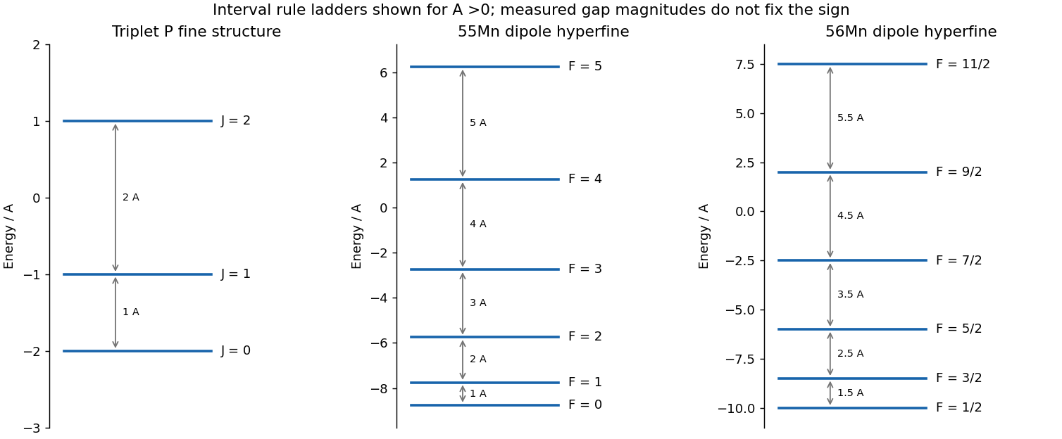
Fine-structure and magnetic-dipole hyperfine interval ladders
. Original angular-momentum eigenvalues for positive coupling coefficients. The fine-structure gaps are A and2A; the two hyperfine examples have different lowest total angular momenta. Measured positive gaps alone do not fix the coupling signs. Details. Past exam of the quantum, atomic and molecular physics course of the University of Oxford 2016 2 a Solution by Codex 0 2026-10-25
Codex 0 2026-10-25First make the units explicit. Use angular momentum operators in units of , so their squared eigenvalues are rather than ; the coefficient then has units of energy. The operator identitygives, at fixed ,Subtracting the expression for the adjacent allowed value leavesThis is the Landé interval rule. Its content is that consecutive gaps grow in proportion to the higher total-angular-momentum quantum number, with the same coefficient within an isolated coupled multiplet. A negative reverses the ordering of the levels, while positive observed transition frequencies alone measure gap magnitudes.
If the source symbols instead denote physical angular momenta with units of action, the Hamiltonian written literally as gives the gap . Recovering the printed form then requires absorbing into the coefficient or writing . The convention is essential to dimensional consistency rather than an extra dynamical assumption.
Past exam of the quantum, atomic and molecular physics course of the University of Oxford 2016 1 d Solution by Codex 0 2026-10-25
Codex 0 2026-10-25In the regime of weak-field Zeeman splitting, remain good labels and . For the 393.4 nm line, in and in . The Landé g-factors are and . Apply to the four upper and two lower sublevels. The allowed pairs areTheir frequency displacements in units of are respectively , so none coincide. Looking perpendicular to the field permits both the radiation from transitions and the radiation from transitions. ConsequentlyA linear polarizer parallel to the field isolates the two components; a transverse polarizer selects the four components. Without polarization selection both sets are present. This count assumes a field small compared with fine structure coupling and neglects isotope-dependent hyperfine structure; the strong-field Paschen-Back effect or a resolved nonzero-spin isotope would require a different model. The spectral spacings are unnecessary for the count, but the distinct shifts verify that counting allowed transitions does not inadvertently count degenerate lines twice.
Past exam of the quantum, atomic and molecular physics course of the University of Oxford 2016 1 c Solution by Codex 0 2026-10-25
Codex 0 2026-10-25The limit near 121.8 nm lies about eV above its lower term. Subtracting from the approximately eV ground-state ionization energy puts that lower term near eV: the pair. The first upper levels are the already identified pair. Their allowed decays areThe fourth possible pairing, , has and is forbidden as an electric dipole transition. The three lines therefore arise from doublet terms, not a spin-triplet term: “triplet series” counts three spectral lines.
For example, the first two wavelengths together with the energy give eV and eV. The longer 854.2 nm wavelength from the same upper level places its lower D level higher. The 866.2 nm transition independently returns the lower D energy within the rounding precision. Increasing the upper principal quantum number gives triplets with two nearby lower-term ionization limits near 121.8 nm. The arrows are included in b; their emission direction is P to D, not the reverse. The independent tabulation confirms the D-term position and ordering.[ref]
Energy Levels of Singly Ionized Calcium (Ca II) by National Institute of Standards and Technology. 3d entries at13650.20 and13710.89 inverse centimetres
Pinned article: Introduction to the OurBigBook Project
Welcome to the OurBigBook Project! Our goal is to create the perfect publishing platform for STEM subjects, and get university-level students to write the best free STEM tutorials ever.
Everyone is welcome to create an account and play with the site: ourbigbook.com/go/register. We belive that students themselves can write amazing tutorials, but teachers are welcome too. You can write about anything you want, it doesn't have to be STEM or even educational. Silly test content is very welcome and you won't be penalized in any way. Just keep it legal!
Intro to OurBigBook
. Source. We have two killer features:
- topics: topics group articles by different users with the same title, e.g. here is the topic for the "Fundamental Theorem of Calculus" ourbigbook.com/go/topic/fundamental-theorem-of-calculusArticles of different users are sorted by upvote within each article page. This feature is a bit like:
- a Wikipedia where each user can have their own version of each article
- a Q&A website like Stack Overflow, where multiple people can give their views on a given topic, and the best ones are sorted by upvote. Except you don't need to wait for someone to ask first, and any topic goes, no matter how narrow or broad
This feature makes it possible for readers to find better explanations of any topic created by other writers. And it allows writers to create an explanation in a place that readers might actually find it.
Figure 1. Screenshot of the "Derivative" topic page. View it live at: ourbigbook.com/go/topic/derivativeVideo 2. OurBigBook Web topics demo. Source. - local editing: you can store all your personal knowledge base content locally in a plaintext markup format that can be edited locally and published either:This way you can be sure that even if OurBigBook.com were to go down one day (which we have no plans to do as it is quite cheap to host!), your content will still be perfectly readable as a static site.
- to OurBigBook.com to get awesome multi-user features like topics and likes
- as HTML files to a static website, which you can host yourself for free on many external providers like GitHub Pages, and remain in full control

Figure 2. You can publish local OurBigBook lightweight markup files to either OurBigBook.com or as a static website.
Figure 3. Visual Studio Code extension installation.
Figure 5. . You can also edit articles on the Web editor without installing anything locally. Video 3. Edit locally and publish demo. Source. This shows editing OurBigBook Markup and publishing it using the Visual Studio Code extension. 
- Infinitely deep tables of contents:




All our software is open source and hosted at: github.com/ourbigbook/ourbigbook
Further documentation can be found at: docs.ourbigbook.com
Feel free to reach our to us for any help or suggestions: docs.ourbigbook.com/#contact