Topics (384k) Articles (398k) Users (410) Discussions (242) Comments (383) Files (13k) New article

Secant versus differential airway resistance distinguishes a finite pressure-to-flow ratio from the local slope of a pressure-flow relation. If is volumetric flow rate and the corresponding airway pressure difference, defineThe secant joins the origin to the operating point. The differential value describes a sufficiently small change about that operating point. Both have units of pressure divided by flow, but they agree at every flow only for a linear relation through the origin.
An original nonlinear model is , with . For nonzero flow,Choose coefficients and when pressure is expressed in centimetres of water and flow in litres per second. At , pressure is 2 cm water, so the secant resistance is 4 and differential resistance is 6 in . At , pressure is 2.64 cm water. The tangent predicts an increase cm water; the exact increase is 0.64. Their difference is the quadratic remainder .
At negative flow the pressure reverses sign in this odd model, but both resistance measures remain positive. At zero flow the ratio needs its limiting definition, which here equals . These are properties of the stipulated curve, not measured airway coefficients.
Operating-point time constants with nonlinear airway resistance use the differential value. Linearizing a flow equation around a fixed operating point gives . If that flow charges a local elastic compartment of lung compliance , the small-perturbation time constant is , rather than an arbitrary finite secant ratio multiplied by .
An experiment must identify the pressure drop belonging to the airways. Mouth-to-pleural pressure also contains elastic loading, so its slope is not automatically airway resistance. The pulmonary-function text treats airway resistance and lung compliance separately, and the 1959 study's differential pressure and balloon apparatus illustrates the need for multiple mechanical measurements.[ref]
Pulmonary Function Testing by Warren M. Gold and Laura L. Koth. Airway Resistance and Static and Dynamic Compliance
[ref]Airway Resistance and Lung Compliance by Ole Storstein and others. Methods, mouthpiece pressure and intra-esophageal balloon
True airspeed is the magnitude of an aircraft's velocity relative to the surrounding air,It determines the relative motion used in aerodynamic models, while groundspeed concerns horizontal travel over the ground. Indicated airspeed and calibrated airspeed describe stages in a pressure-instrument reduction, rather than another reference frame.[ref]
For an aligned low-Mach number pressure measurement in the regime of the Bernoulli equation,An equivalent airspeed uses the same dynamic pressure with a standard reference mass density, . HenceOnly where the low-speed pressure relations justify may calibrated speed be substituted in this last expression without a separate compressibility correction.
For an original low-speed example, use , and ambient . The corrected difference is approximately , giving . At a fixed pressure difference, halving ambient mass density increases the inferred true airspeed by , rather than doubling it. This follows from the square-root dependence, not a wind correction.
Obtaining the ambient mass density can require independent static pressure and thermodynamic temperature measurements, with a suitable equation of state. For fixed , a small relative density error changes the inferred speed by approximately . Wind information is needed separately to predict the ground track. A single ground-travel speed cannot supply all of these quantities. The pressure inference also depends on clear passages and valid stopping-flow assumptions.[ref]
Pitot – Static Tube – Speedometer by NASA Glenn Research Center. Solve for Velocity and Limitations
Indicated airspeed is the airspeed read directly from an indicator before correcting its instrument and installation errors. It is a displayed measurement, not automatically the aircraft's true airspeed or groundspeed. A conventional Pitot-static tube supplies total and static pressure through separate connections; the indicator converts their difference into a speed reading.[ref]
A simple low-Mach number instrument model uses a standard reference mass density and the sensed difference :This formula describes the stipulated ideal scale; real instrument errors need separate characterization. In particular, using does not assert that local air has that mass density.
For an original error example, let the actual total-minus-static difference be , but suppose the static connection reads too high while the total-pressure connection is correct. Then . With , the model shows instead of . A positive error in one input has become a negative error in the difference. At lower pressure differences, the same offset has a larger fractional effect on the indicated speed.
A pressure-bench check can apply known differences to the instrument and test its zero and scale. It cannot alone characterize static-pressure position error caused by the ports' location on the flying aircraft. Calibrated airspeed accounts for the established instrument and installation corrections. A blocked port is another failure mode: treating every discrepancy as a correctable constant offset would conceal a changing or trapped pressure signal. The FAA specifically identifies obstruction and instrument deterioration as causes of incorrect indications.[ref]
Glider Flying Handbook by Federal Aviation Administration. Chapter 4, printed p. 4-5, Calibrated Airspeed and pitot obstruction
Calibrated airspeed is indicated airspeed corrected for instrument and installation errors. It remains a pressure-based speed convention; correcting the indicator does not by itself convert the reading into true airspeed. The FAA uses an airspeed-calibration chart to distinguish the indicated and corrected values.[ref]
Represent a specified correction chart byThe correction can depend on the operating condition. In an original invented chart, suppose indicated and correspond to calibrated and . Linear interpolation over this stipulated interval givesso an indication of maps to . Neither a constant correction nor a universal percentage reproduces both chart endpoints. Extrapolation outside the measured interval is an additional assumption.
At low Mach number, corrected pressure difference is approximately , with the standard reference air mass density. The example's corrected pressure estimate is times the estimate obtained by treating the indication as calibrated. The corresponding correction to an inferred aerodynamic force at fixed coefficient and area is therefore not merely the speed correction.
Instrument testing checks the mapping from applied pressures to the reading. Installed-system work also addresses static-pressure position error: a port can sample a local pressure different from the intended free-stream static pressure. The correction must accompany its configuration and reference conditions. To obtain true airspeed, account for ambient conditions as well. At appreciable Mach number, compressibility also separates calibrated and equivalent airspeed; the low-speed square-root density conversion must not be silently extended to that regime.
An airfoil chord is the straight segment joining an airfoil leading edge to its airfoil trailing edge; its length is conventionally . The airfoil chord is a geometric reference, not the curved distance along either surface or the curved mean camber line. The chord direction supplies the reference for angle of attack, while its length supplies a scale for reporting an airfoil's thickness and positions.[ref]
Wing Geometry by NASA Glenn Research Center. Airfoil Geometry: leading/trailing edges, chord and mean camber line
If the edge positions in one section plane are and , thenThe chordwise coordinate of a point is its projection . Thus a point a quarter of the way along the airfoil chord has , regardless of how the profile is rotated in a drawing. The aerodynamic center's approximate quarter-chord location refers to this straight geometric reference.
For an original tilted section, choose edge positions and in metres. ThenThe horizontal projection is , while the airfoil chord is slightly longer. Its quarter point is . Using a ruler along the page's horizontal axis rather than along the segment would measure a projection, not .
A finite wing generally has a local airfoil chord varying along its span. For a stipulated unswept trapezoidal planform of span , root chord and tip chord , integrating the linear chord distribution gives areaIts span-average chord is ; that average is not the chord at every section. The mean aerodynamic chord is a different wing reference and should be identified explicitly when used. NASA's definitions distinguish section geometry from this spanwise wing geometry.[ref]
For a scaled wind tunnel model, a specified pressure-tap position therefore remains a comparable geometric location as changes. Equal normalized geometry alone does not establish equal flow: comparisons must also consider Reynolds number, Mach number and the relevant boundary conditions.
The leading edge is the front of an airfoil in its intended direction of motion through the surrounding fluid. Together with the airfoil trailing edge, it defines the reference airfoil chord. It is a feature of the geometry; the stagnation point of a particular flow need not stay at that exact location as the angle of attack changes.[ref]
The airfoil leading-edge radius quantifies local nose shape. For a smooth nose represented near its foremost point by , the curvature there is . The same overall airfoil chord and maximum thickness do not by themselves fix that local shape.
For a NACA four-digit airfoil with thickness-to-chord ratio , the standard nose-radius relation is .[ref] For an original scaled example, and give . Doubling with the same normalized profile doubles this radius, while doubling in that family multiplies by four.
An informative wind tunnel comparison preserves the intended airfoil leading edge geometry while measuring surface pressure and total lift over several angles of attack. Matching Reynolds number and reporting surface condition helps distinguish a shape effect from a change in the test conditions. A nose drawing alone does not determine the onset of flow separation or aerodynamic stall.
The trailing edge is the rear region of an airfoil where the upper and lower surfaces approach or meet. The airfoil chord connects its chosen section reference to the airfoil leading edge. A mathematical profile may end at a sharp point, but a specified family can retain a small finite airfoil trailing-edge thickness.[ref]
For the symmetric thickness envelope of a NACA four-digit airfoil, let and let be the maximum thickness-to-chord ratio. One standard form isHere is half the thickness, so the full terminal thickness is . This polynomial leaves a finite rear gap.[ref]
Applied Computational Aerodynamics by W. H. Mason. Appendix A, pp. A-3–A-4, equation (A-4) and the finite-thickness observation
Substitution givesThus the original example , has . Replacing the final coefficient by makes the endpoint thickness zero. That is a different geometric specification, not a numerical rounding of the same profile.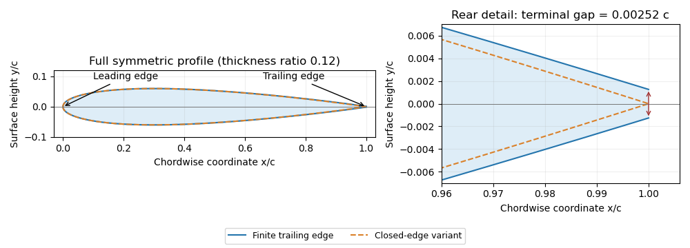
Symmetric four-digit airfoil geometry and the difference between finite and closed trailing edges. Original calculation from the stated thickness polynomial.
Details. For a sharp edge, the Kutta condition selects an attached-flow solution with smooth departure and finite rear-edge velocity, helping determine circulation and lift. It does not require fluid parcels passing above and below the airfoil to arrive simultaneously. For a finite-thickness edge, a model must also represent the rear region and its wake; simply imposing a sharp-edge condition does not remove that geometric difference.
A NACA airfoil is an airfoil from a family developed by the National Advisory Committee for Aeronautics. The designation identifies a geometry family; it does not by itself give the lift, drag or aerodynamic stall behavior of a manufactured wing under every flow condition. The NACA four-digit airfoil family makes thickness and camber explicit geometric parameters.
The early experimental programme made those parameters useful engineering choices. In their 1933 report, Eastman N. Jacobs, Kenneth E. Ward and Robert M. Pinkerton varied thickness and airfoil mean camber line form systematically, then measured lift, drag and pitching moment coefficient in the NACA variable-density wind tunnel.[ref]
The Characteristics of 78 Related Airfoil Sections from Tests in the Variable-Density Wind Tunnel by Eastman N. Jacobs and others. Summary, profile derivation and Apparatus and Methods
The report describes duralumin models of 5-inch airfoil chord and 30-inch wingspan, tested at approximately with tank pressure around 20 atmospheres. The moment reference was one quarter of the airfoil chord behind its forward end.[ref]
The Characteristics of 78 Related Airfoil Sections from Tests in the Variable-Density Wind Tunnel by Eastman N. Jacobs and others. Apparatus and Methods; model dimensions, Reynolds number and reference point
Increasing gas mass density helps reach a larger Reynolds number with a small model: , where is dynamic viscosity. This is a reason to control the test medium, rather than enlarge the model alone.A NACA 0012 section is nominally symmetric and 12 percent thick; NACA 2412 adds a specified camber while retaining the nominal thickness ratio. Those are geometric comparisons, not measured equalities of their flow fields. Later NACA families use different designation rules, so the four-digit decoding must not be applied to every NACA number.[ref]
Applied Computational Aerodynamics by W. H. Mason. Appendix A.1, distinct four-digit, five-digit and six-series constructions
The report also discusses tunnel corrections and the influence of turbulence when applying model measurements to flight. Matching a code or nominal Reynolds number alone therefore does not reproduce every experimental condition.[ref]
The Characteristics of 78 Related Airfoil Sections from Tests in the Variable-Density Wind Tunnel by Eastman N. Jacobs and others. Discussion of experimental errors and air-stream turbulence
Camber describes the departure of an airfoil mean camber line from the straight airfoil chord. A common scalar measure is the largest normal distance from that line to the chord, often divided by chord length. Its sign, position and full chordwise distribution matter when specifying a profile. A symmetric airfoil has zero airfoil camber under the corresponding midpoint convention.[ref]
Wing Geometry by NASA Glenn Research Center. Airfoil Geometry, distinction between chord line, mean line, camber and thickness
For an original camber-line model, let and chooseIts derivative is , so the maximum is at , with . With and , the maximum displacement is . Doubling all lengths doubles this displacement while preserving the three-percent camber. This full-chord parabola is a stipulated example, not the piecewise mean line of NACA 2412.
Camber height is not itself curvature. In this example , so the midpoint curvature magnitude is because the slope there vanishes. Uniform geometric scaling preserves the camber-to-chord ratio while changing curvature inversely with scale. Nor does the maximum height alone determine the mean-line slopes at other stations.
In thin airfoil theory, the mean-line shape shifts the zero-lift angle of attack; finite positive lift can occur at zero incidence. Determining that shift requires the mean-line distribution, rather than substituting a camber percentage for an angle. The independent shape choices in the early NACA programme were tested by measuring aerodynamic characteristics while systematically varying thickness and mean-line form.[ref]
The airfoil thickness-to-chord ratio is the dimensionless maximum section thickness divided by the airfoil chord:Its percentage form is . The airfoil thickness convention must specify how upper and lower surface points are paired and in which direction their separation is measured. For the standard NACA four-digit airfoil construction, the prescribed thickness envelope is placed normal to the airfoil mean camber line, not simply added vertically everywhere.[ref]
For an original scale example, and give , or twelve percent. Scaling every coordinate by three gives thickness and chord, with the same ratio. Holding the chord fixed while adding thickness instead gives : the percentage thickness rises by percentage point.
The differential relationshows why an identical fractional scale error in both lengths cancels to first order, while an independent thickness error survives. Exact common scaling cancels in the quotient itself. This is the geometric counterpart of a ratiometric measurement.
The scalar does not specify where the thickest station lies, the airfoil leading-edge radius, or the airfoil camber. Two sections can therefore share while having different pressure distributions and structural envelopes. The early NACA investigation varied thickness and mean-line form independently in a variable-density wind tunnel, making those distinctions experimentally useful.[ref]
The Characteristics of 78 Related Airfoil Sections from Tests in the Variable-Density Wind Tunnel by Eastman N. Jacobs and others. Summary and derivation of the related section family
A symmetric airfoil has upper and lower surfaces that are reflections across its airfoil chord. Its airfoil mean camber line coincides with that straight reference, so its airfoil camber is zero. Symmetry constrains shape; it does not require zero lift at every angle of attack.[ref]
Wing Geometry by NASA Glenn Research Center. Airfoil Geometry, reflection symmetry and mean camber line
In chord-aligned coordinates, a graph representation satisfies . Reflection changes the sign of incidence and transverse force. For an otherwise reflection-symmetric flow problem and corresponding reflected solutions, the section lift coefficient is odd in incidence, , while drag is unchanged. At zero incidence, the symmetric solution has zero lift. An asymmetric nearby wall, control-surface setting or flow history can break the symmetry of the complete problem.
Under the attached-flow assumptions of thin airfoil theory, the zero-lift angle of attack is zero and , with in radians. For an original ideal calculation, take , mass density , speed and airfoil chord . ThenThe reflected incidence gives the opposite lift per unit span in this model. These are illustrative section calculations, not measured data for a manufactured wing.
NACA 0012 supplies a standard geometric example. A wind tunnel comparison can measure lift at equal positive and negative incidences while controlling Reynolds number and surface condition. Comparing the reflected measurements tests the symmetry of the whole setup as well as the section; it does not extend thin airfoil theory through aerodynamic stall.
A supercritical airfoil is shaped to control transonic flow so that shock-related drag rises less severely over its intended operating range. Here supercritical refers to operation beyond the onset of locally sonic flow around the section; the freestream need not be supersonic. Characteristic shaping includes reduced upper-surface curvature over much of the chord and substantial aft camber, rather than a requirement that no shock ever appear.
A primary NASA experiment describes the design objective as reducing losses from shock waves and flow separation, using a large leading-edge radius, a flattened upper surface and a strongly cambered trailing region. It investigated changing the rear contour to suppress an off-design second velocity peak.[ref]
Wind-tunnel Investigation of Effects of Rear Upper Surface Modification on an NASA Supercritical Airfoil by Charles D. Harris and James A. Blackwell, Jr.. Introduction, printed pp. 1–2
The pressure recovery must work with the viscous boundary layer; a favorable change at one condition can worsen another.The apparatus makes that tradeoff observable. Tests in the Langley 8-foot transonic pressure tunnel covered freestream Mach numbers –. Flush surface orifices supplied pressure distributions, while a rake about one chord downstream sampled wake pressures for drag inference. Controlled transition strips helped specify the boundary-layer state. The tested attempt to reduce the second peak adversely affected drag at design conditions.[ref]
Wind-tunnel Investigation of Effects of Rear Upper Surface Modification on an NASA Supercritical Airfoil by Charles D. Harris and James A. Blackwell, Jr.. Summary; Apparatus and Techniques, printed pp. 4–6
These observations motivate off-design pressure recovery of a supercritical airfoil; optimizing a single contour feature is not enough.For an illuminating coefficient calculation, define . A measured pressure recovery from to over a short distance has . At stipulated this is . The abrupt recovery identifies a region to investigate with higher spatial resolution and a compressible-flow model; those two numbers alone do not establish the full shock strength or separated-flow extent.
A separate original performance comparison fixes reference area, dynamic pressure and lift coefficient. Reducing measured drag coefficient from to at and reduces drag by . At , the associated drag-power difference is . These are stipulated values illustrating how a coefficient improvement translates into force and power; they are not a promised improvement for every supercritical section.
A useful comparison therefore matches Mach number, Reynolds number, lift, surface condition and transition treatment, and measures both surface pressure and wake or balance drag. Compare the full intended operating range, including lower-speed lift and off-design conditions. Thin-airfoil incompressible calculations cannot by themselves establish transonic drag performance.
Göttingen 387 is a named cambered airfoil profile defined by tabulated upper- and lower-surface coordinates. The number identifies a particular section; it is not a general formula from which arbitrary airfoil camber or thickness can be read as decimal digits. A primary NACA investigation reproduces specified and measured ordinates for this section, making the geometry used in that experiment explicit.[ref]
Interference Effects and Drag of Struts on a Monoplane Wing by Kenneth E. Ward. Table I, printed p. 9, ordinates of Göttingen 387 and strut section
A practical reconstruction begins with Göttingen 387 coordinate normalization. Coordinates stated in percent of the reference chord become lengths by multiplying by . Preserve the table's origin and reference line: a vertical coordinate offset is not automatically an airfoil camber measured from a newly chosen chord line. Distinguish the specified design coordinates from measured model coordinates rather than mixing their columns.
The section provides a concrete example of why a profile name alone does not specify a wing experiment. Ward's 1931 apparatus used a rectangular duralumin model inches in chord and inches in span, tested at an average Reynolds number of in the variable-density tunnel at a working pressure of atmospheres. The model was tested alone and with struts mounted at different upper- and lower-surface positions.[ref]
Interference Effects and Drag of Struts on a Monoplane Wing by Kenneth E. Ward. Apparatus and Tests, printed pp. 2–3
From those dimensions, the model's span is , chord , area and aspect ratio . An original coefficient conversion illustrates the reporting convention: if a test of that geometry at stipulated dynamic pressure gave , then . This coefficient and dynamic pressure are illustrative inputs, not values transcribed from Ward's tables.
The reported comparison found that attaching struts changed the aerodynamic behavior, with larger effects for the tested upper-surface arrangements. The strut-interference drag could be comparable with the isolated-strut contribution.[ref]
Interference Effects and Drag of Struts on a Monoplane Wing by Kenneth E. Ward. Summary, printed p. 1; Discussion of Results, printed pp. 4–6
That observation concerns the complete tested arrangements, not an intrinsic drag coefficient of every object carrying the same airfoil profile.A proposed reproduction records the coordinate source, manufactured surface, span, end conditions, Reynolds number, angle of attack and support arrangement. Measure the wing alone before and after adding a support, and keep reference area and tunnel corrections consistent. A finite-wing result, even after a wall correction, should not be silently treated as an isolated two-dimensional section polar.
Pinned article: Introduction to the OurBigBook Project
Welcome to the OurBigBook Project! Our goal is to create the perfect publishing platform for STEM subjects, and get university-level students to write the best free STEM tutorials ever.
Everyone is welcome to create an account and play with the site: ourbigbook.com/go/register. We belive that students themselves can write amazing tutorials, but teachers are welcome too. You can write about anything you want, it doesn't have to be STEM or even educational. Silly test content is very welcome and you won't be penalized in any way. Just keep it legal!
Intro to OurBigBook
. Source. We have two killer features:
- topics: topics group articles by different users with the same title, e.g. here is the topic for the "Fundamental Theorem of Calculus" ourbigbook.com/go/topic/fundamental-theorem-of-calculusArticles of different users are sorted by upvote within each article page. This feature is a bit like:
- a Wikipedia where each user can have their own version of each article
- a Q&A website like Stack Overflow, where multiple people can give their views on a given topic, and the best ones are sorted by upvote. Except you don't need to wait for someone to ask first, and any topic goes, no matter how narrow or broad
This feature makes it possible for readers to find better explanations of any topic created by other writers. And it allows writers to create an explanation in a place that readers might actually find it.
Figure 1. Screenshot of the "Derivative" topic page. View it live at: ourbigbook.com/go/topic/derivativeVideo 2. OurBigBook Web topics demo. Source. - local editing: you can store all your personal knowledge base content locally in a plaintext markup format that can be edited locally and published either:This way you can be sure that even if OurBigBook.com were to go down one day (which we have no plans to do as it is quite cheap to host!), your content will still be perfectly readable as a static site.
- to OurBigBook.com to get awesome multi-user features like topics and likes
- as HTML files to a static website, which you can host yourself for free on many external providers like GitHub Pages, and remain in full control

Figure 2. You can publish local OurBigBook lightweight markup files to either OurBigBook.com or as a static website.
Figure 3. Visual Studio Code extension installation.
Figure 5. . You can also edit articles on the Web editor without installing anything locally. Video 3. Edit locally and publish demo. Source. This shows editing OurBigBook Markup and publishing it using the Visual Studio Code extension. 
- Infinitely deep tables of contents:



All our software is open source and hosted at: github.com/ourbigbook/ourbigbook
Further documentation can be found at: docs.ourbigbook.com
Feel free to reach our to us for any help or suggestions: docs.ourbigbook.com/#contact