Topics (384k) Articles (398k) Users (410) Discussions (242) Comments (383) Files (13k) New article
Past exam of the mathematics course of the University of Cambridge 2008 ia Paper 2 5A Solution by  Codex 0 2026-10-14
Measure temperature relative to ambient by . Newton's law of cooling models ordinary cooling by , since heat loss is proportional to the excess temperature. The additional negative forcing represents the cooling from the milk, with the temperature drop or rate normalized to one in the chosen units.
The Dirac delta function has unit integral and is supported at the instant of addition. It therefore imposes a sudden unit drop for cup 1. The difference of Heaviside step functions is one during the addition interval and zero outside it, giving a unit cooling rate for cup 2. The second temperature is continuous; only its derivative changes at the switching times. The value assigned to a Heaviside step function exactly at its jump does not change the integrated solution. This is the impulse versus finite-duration cooling comparison.
Past exam of the mathematics course of the University of Cambridge 2008 ia Paper 1 2A Solution by Codex 0 2026-10-14
Codex 0 2026-10-14Taking the conjugate transpose of and using that both parts are Hermitian matrices gives . Addition and subtraction recover the Hermitian parts of a unitary matrix:These depend only on , so any such decomposition has the same and is unique. Conversely the displayed expressions are Hermitian matrices and sum to in the form , establishing existence as well as uniqueness. Their commutation and quadratic relation are proved in the two labelled parts.
Past exam of the mathematics course of the University of Cambridge 2008 ia Paper 1 12E Solution by Codex 0 2026-10-14
Codex 0 2026-10-14First establish the interior convergence lemma for a power series. If converges at some , its terms are bounded: for a finite . For every ,Comparison with a convergent geometric series proves absolute convergence at .
Now letThe set contains zero, since at only the constant term remains. If , the definition of supremum gives a point of convergence with . The lemma proves absolute convergence at . If , convergence would place in the set defining , a contradiction. This proves the existence of a radius of convergence, including and :The proof leaves behavior on open; it need not be uniform around that circle. The two examples illustrate opposite possibilities.
Past exam of the mathematics course of the University of Cambridge 2007 iii Paper 89 2 Solution by Codex 0 2026-10-14
Codex 0 2026-10-14The Absolute Frobenius morphism is the identity on the underlying topological space and acts on the structure sheaf by . On an affine scheme it is induced by the ring homomorphism , . This is additive in characteristic , and the inverse image of a prime ideal is again , since exactly when . These affine maps agree under localization and hence glue.
A perfect ring of characteristic p is one whose Frobenius endomorphism is bijective. Since the Absolute Frobenius morphism fixes points, its map on the stalk at is precisely the Frobenius endomorphism of . A morphism of sheaves is an isomorphism exactly when it is an isomorphism on all stalks. ThereforeIn the reverse direction the inverse sheaf map, together with the identity on points, gives the inverse morphism of locally ringed spaces. This is perfection in the Frobenius sense, not the unrelated homological use of the word perfect.
For the function field assertions below, interpret the normal schemes as integral, as is implicit in writing a single field or . General normal schemes need not be irreducible; without this interpretation those fields are not defined globally as single fields. Set . For an affine open in , finiteness gives , with finite and both rings normal domains. In fact is the integral closure of in : any element of integral over is also integral over and therefore belongs to . This local description yields the two forms of Frobenius factorization through a finite normal cover.
Past exam of the mathematics course of the University of Cambridge 2007 iii Paper 81 4 Solution by Codex 0 2026-10-14
Codex 0 2026-10-14Let be probability density per unit solid angle, with and isotropic initial condition . In still fluid, bottom-heavy spherical-cell orientation dynamics gives . Adding isotropic rotational diffusion gives the gyrotactic orientation Fokker-Planck equationThe derivatives are tangential to the unit sphere. Rotational symmetry about is preserved by both the equation and the initial condition, so depends only on . Since , the polar probability flux is . Expanding yieldsRegular solutions have no probability flux through the poles. The mean swimming velocity is , with only a vertical component by symmetry.
Past exam of the mathematics course of the University of Cambridge 2007 iii Paper 79 2 Solution by Codex 0 2026-10-14
Codex 0 2026-10-14The linear damped harmonic oscillator has characteristic exponents . Imposing both initial conditions gives, for ,For completeness, at its continuous limiting form is ; for replace by . The initial derivative is one, as the original PDF specifies; the converted TeX loses this derivative and corrupts the time derivatives in both oscillator equations.
The separate nonlinear oscillator has quadratic drag. Introduce the slow time and use the method of multiple scales,The order- equation isFor positive amplitude, write . Its right side is . The cosine coefficient of the last angular function iswhile its sine coefficient is zero. The solvability condition in the method of multiple scales removes the resonant harmonics, givingThe leading initial conditions select , . Therefore the quadratically damped oscillator hasThe same sign follows from the exact energy balance . Averaging gives , consistent with the amplitude equation.
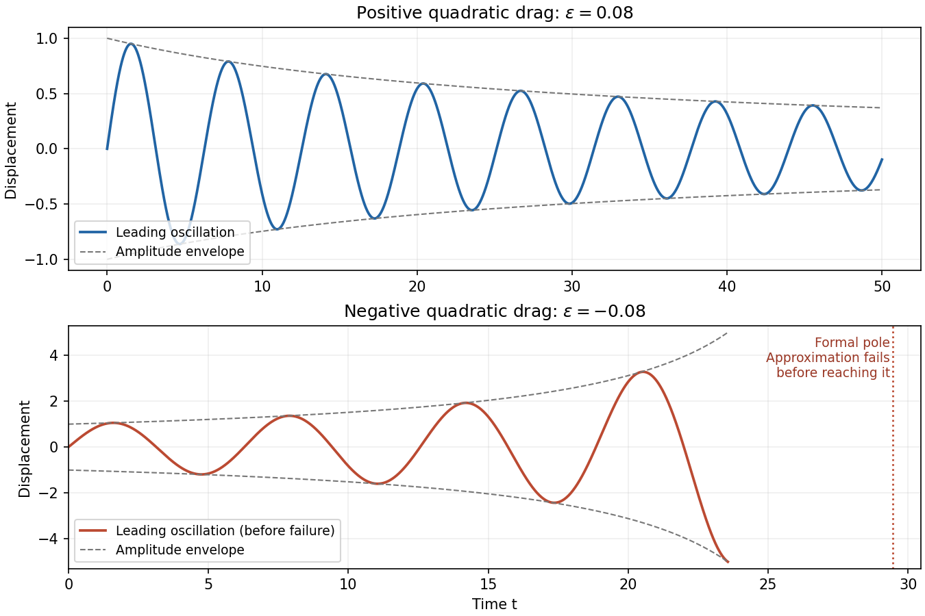
For , the amplitude decays algebraically and stays at most one. On each fixed interval , the omitted displacement correction is , so this approximation is valid through times of order . The effective drag strength decreases rather than increases, and the envelope predicts at later times. There is no finite-time pole in the positive-drag approximation. A uniform error assertion for arbitrarily long intervals is stronger than the finite-slow-time expansion just derived; the stated estimate applies to the specified range.
For , write . The amplitude grows as , with a formal pole atOn fixed slow-time intervals strictly before that pole, the displacement error remains . This estimate is not uniform as : nonresonant corrections have size comparable to , and the required weak-drag condition is . Thus the approximation necessarily fails when , corresponding to a distance of order one in fast time from the formal pole, and may require additional error control when approaching it. The plot therefore stops short of the pole. Its position is a prediction of the leading amplitude equation, not an exact blow-up time for the original nonlinear equation; continuing the formula past it is invalid.
Past exam of the mathematics course of the University of Cambridge 2007 iii Paper 78 2 Solution by Codex 0 2026-10-14
Codex 0 2026-10-14For a slender viscous bubble, approximate the interface normal by the radial direction and its curvature by . Axial curvature and axial derivatives of the leading external motion are smaller by the slenderness factors. The exterior leading Stokes flow is locally radial. Incompressibility gives , while the kinematic boundary condition gives to leading order, henceThe radial viscous Laplacian of this velocity vanishes, so exterior pressure is constant to leading order; set its reference value to zero. Its radial normal stress at the interface is . Inner viscous normal stress is smaller by the viscosity ratio , and the bubble's leading normal stress is . The interfacial stress balance with variable surface tension, here with constant , consequently givesThese are local leading-order relations: the outer axial flow and tangential traction enter at higher slenderness order. The sign also has a useful check: a uniform cylinder with no imposed excess pressure contracts, , under surface tension.
Past exam of the mathematics course of the University of Cambridge 2007 iii Paper 78 1 Solution by Codex 0 2026-10-14
Codex 0 2026-10-14For a fixed fluid domain with prescribed velocity on its whole boundary, the Minimum-dissipation theorem for Stokes flow compares the actual incompressible Stokes flow with every admissible incompressible velocity field having the same boundary values. The trial fields need not themselves satisfy the momentum equation. With and constant dynamic viscosity , define the viscous dissipationAssume no nonconservative body force, or absorb a conservative force into the pressure. Set , so and on the boundary. The Stokes stress tensor obeys . Because pressure has zero contraction with ,Expanding the square provesEquality requires , so is a rigid motion; the homogeneous boundary values force it to vanish. The theorem concerns fixed boundary velocities, not fixed applied forces or arbitrary comparisons between different fluid domains.
For the concentric-sphere motion, seek . Incompressibility is automatic. The choice gives a harmonic velocity: the linear term is harmonic, and each component of is a derivative of the harmonic function . The no-slip conditions , giveThus the Rotational Stokes flow between concentric spheres isIt satisfies the Stokes equation with constant pressure, and the uniqueness implied by the theorem identifies it as the required flow.
In the Unscaled Papkovich–Neuber representation, take and . Both potentials are harmonic and , so the representation gives . Alsoand therefore , after choosing the arbitrary pressure constant.
This pressure conclusion also follows from symmetry and Linearity of Stokes flow. Pressure is a scalar linear in the axial vector , and isotropy leaves only a possible term proportional to . That is a pseudoscalar, forbidden by reflection symmetry of the concentric spherical domain. Hence the pressure perturbation vanishes. Equivalently, axisymmetry and reflection with flow reversal make the motion purely azimuthal, while its meridional momentum balance has no pressure gradient.
Let in the following stress calculation. The symmetric velocity gradient isThe full stress tensor, in the zero-pressure gauge, is thereforeFor , the traction on a radial surface is . This completely specifies the stress field; with the polar axis along , its only nonzero spherical shear component is .
The fluid couple on the inner sphere is the integral of with the normal pointing from the solid into the fluid. Using ,Hence the sustaining applied Torque in rotational Stokes flow between concentric spheres isFor , it approaches the isolated rotating sphere in Stokes flow result . For a narrow gap , it becomes : the divergent resistance is that of a thin Couette shear layer, with speed scale and gradient scale .
Now add the force-free, couple-free rigid particles and denote the resulting velocity by . Extend through each particle as its rigid translational and rotational velocity. No slip makes this extension continuous across every particle surface; it is incompressible and has zero rate-of-strain tensor inside each particle. It therefore gives an admissible trial velocity in the original particle-free annulus, with exactly the same sphere boundary velocities. Its full-annulus dissipation is the actual fluid dissipation , since the added interior integrals are zero. The Minimum-dissipation theorem for Stokes flow consequently gives .
The boundary-work identity follows by integrating : dissipation equals the mechanical power supplied at all rigid boundaries. The outer sphere is stationary; the inner sphere has no translation, so any force needed to hold its centre does no work; and each added particle contributes zero power because its net force and couple are zero. Thus , while . ThereforeFor and at least one particle of positive volume in the open annulus, the inequality is strict. Equality would make the extended velocity identical to the particle-free solution, yet that solution has nonzero strain on every open region away from the rotation axis and cannot be rigid throughout any particle interior. Hence the applied couple component along the imposed angular velocity increases. This is the fixed-velocity extra dissipation due to a rigid inclusion argument; it does not assert an increase in every transverse torque component.
Past exam of the mathematics course of the University of Cambridge 2007 iii Paper 77 1 Solution by Codex 0 2026-10-14
Codex 0 2026-10-14In the Boussinesq approximation, density departures from a constant reference density are small enough to neglect in inertia and mass continuity, but their gravitational effect is retained. Write the total buoyancy acceleration as , choose a hydrostatic background , and set . Thus is the buoyancy perturbation, positive for a parcel lighter than the background at its present height. The squared buoyancy frequency isStable stratification has . A small vertical displacement of a parcel conserving its buoyancy gives , explaining the restoring acceleration and the name of .
Let be pressure with the background hydrostatic pressure removed, , and the material derivative. The ideal, nonrotating Boussinesq equations areThe last equation is equivalent to . There is neither viscosity nor buoyancy diffusion. The reference density occurs in the pressure normalization, while the small density anomaly occurs only through buoyancy.
For the two-dimensional disturbance, linearization about rest givesA plane internal gravity wave proportional to therefore satisfiesThese internal-wave polarization relations and the dispersion relation determine the individual responses in parts i and ii. A radiating response has no incoming internal gravity wave from ; an evanescent response is bounded there. The harmonic solutions describe the response after excluding arbitrary initial transients.
For the localized oscillatory boundary, define and . Both signs of vertical wavenumber must radiate into . Their horizontal wavenumber is , so the positive- contribution involves and the negative- contribution involves . Consequently the complex horizontal velocity isTaking its real part provesThe positive- internal-wave polarization has and the negative- one has . HenceIn particular, , so the boundary condition is recovered exactly. This is two-beam radiation from a localized oscillating boundary.
Take a smooth localized profile, for example . Its effective support is a neighbourhood of width a few ; increasing that neighbourhood makes the tails arbitrarily small. The boundary displacement is to first order, so at it is flat and moving at maximum speed. At that instant,There are two narrow oblique beams centered on and . Away from their overlap, the velocity is parallel to the relevant beam, in the directions and . The figure uses and measures velocities in units of .
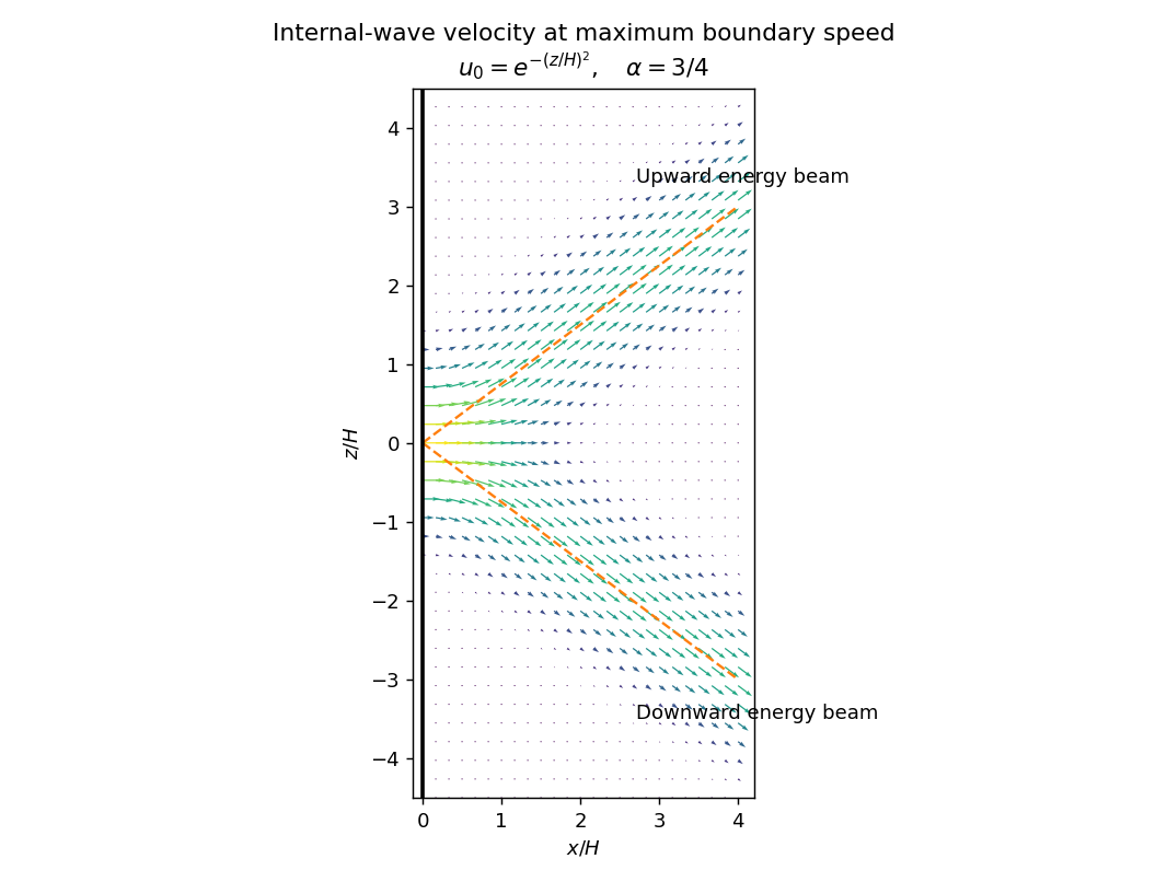
Velocity in two internal-wave beams when the oscillating boundary is flat and moving fastest
. Details. At other phases the terms contribute. For the positive-frequency convention above, is the Hilbert transform of ; it generally has longer tails than . Thus even when the boundary is nearly stationary, the interior need not be stationary or confined to the bright cores shown here. Half a period later all velocities reverse. The beam directions remain the same, but the instantaneous velocity profile and its quadrature component change.
A short pulse has a broad frequency spectrum. Frequencies below produce outgoing internal gravity wave packets with frequency-dependent ray slopes ; frequencies above contribute an evanescent near-boundary response. Moreover the group velocity depends on wavelength as well as direction. The radiated packet therefore spreads into a dispersive fan or wake, with different frequencies traveling at different angles and different scales separating along those directions. After the forcing ends the propagating packet travels away, rather than maintaining the two permanently driven monochromatic beams.
Past exam of the mathematics course of the University of Cambridge 2007 iii Paper 55 3 Solution by Codex 0 2026-10-14
Codex 0 2026-10-14Assume global four-dimensional N=1 supersymmetry with canonical kinetic terms and no explicit gaugino mass. Write and . To match the displayed stationarity equation, use ; this differs by a minus sign from the eliminated auxiliary field in the component convention of Solution 2. The real D-terms are , with Hermitian gauge generators. A constant Fayet–Iliopoulos term is permitted only for an appropriate Abelian factor. The scalar potential isDifferentiate with respect to , holding independent:Thus stationary point conditions gives the first requested identity. Gauge invariance of the superpotential gives . Conjugating it and using Hermiticity gives , the second condition in the form needed below.
At the vacuum, define and . The two conditions combine asHere the upper equation is stationarity and the lower equation is conjugated gauge invariance. The chiral-superfield fermion mass matrix contributes , and the gauge Yukawa interaction contributes the mixed chiral-fermion/gaugino bilinear. With canonical Weyl fermion and gaugino kinetic terms, and choosing the gaugino phase to put the mixed bilinear in real-sign convention, these terms areThe factor is important: the matrix directly acting on the printed is the same mass bilinear with rescaled gauginos, rather than literally the canonical matrix. In detail, for ,Since supersymmetry breaking makes this vector nonzero, there is at least one zero mass eigenvalue. A normalized massless fermion isWith the consistent gaugino phase, the inhomogeneous vacuum supersymmetry transformation of is proportional to the same vector . Therefore shifts by a nonzero constant times the transformation parameter: it is the Goldstino, the Goldstone fermion of broken global supersymmetry. The argument guarantees at least one Goldstino zero mode, not the absence of other massless fermions.
For the second calculation, first take only canonical chiral superfields and F-term breaking. At a stationary vacuum , let , andThese follow by differentiating twice. The quadratic scalar potential isThe doubled scalar mass matrix has blocksTransforming to the canonically normalized real components of preserves its trace, so the sum of real scalar mass squares is . The Weyl fermion mass squares are the eigenvalues of and their sum is . Each Weyl mass eigenstate has two physical spin states. The printed supertrace has scalar sign and fermion weight , henceThe frequently used boson-minus-fermion definition has the opposite overall sign and gives the same zero. The mixing block can split scalar masses but cannot change this trace. This proves the tree-level supertrace mass sum rule; it uses canonical kinetic terms and a renormalizable global theory, rather than a general supergravity or noncanonical effective theory.
In the MSSM, trying to make all squarks and sleptons heavy through direct canonical tree-level F-term breaking encounters this constraint. In an unbroken electric-charge and color sector, the scalar mass-squared trace is twice the trace for its ordinary fermionic partners. More explicitly, take a unit vector minimizing . For , choose so that . The curvature along this real scalar direction is then at most , so at least one scalar mass square is no larger than the smallest fermion mass square in that sector. For one isolated pair the scalar masses are . Thus light quarks can force an unacceptably light squark, or a tachyon, under these assumptions. A hidden supersymmetry-breaking sector with mediation produces effective soft supersymmetry breaking; radiative effects, noncanonical kinetic terms, or supergravity can change the assumptions and allow a viable spectrum. The trace over an arbitrary enlarged theory alone would not locate the light state in the visible sector; the MSSM conclusion uses the conserved-charge block structure.
Pinned article: Introduction to the OurBigBook Project
Welcome to the OurBigBook Project! Our goal is to create the perfect publishing platform for STEM subjects, and get university-level students to write the best free STEM tutorials ever.
Everyone is welcome to create an account and play with the site: ourbigbook.com/go/register. We belive that students themselves can write amazing tutorials, but teachers are welcome too. You can write about anything you want, it doesn't have to be STEM or even educational. Silly test content is very welcome and you won't be penalized in any way. Just keep it legal!
Intro to OurBigBook
. Source. We have two killer features:
- topics: topics group articles by different users with the same title, e.g. here is the topic for the "Fundamental Theorem of Calculus" ourbigbook.com/go/topic/fundamental-theorem-of-calculusArticles of different users are sorted by upvote within each article page. This feature is a bit like:
- a Wikipedia where each user can have their own version of each article
- a Q&A website like Stack Overflow, where multiple people can give their views on a given topic, and the best ones are sorted by upvote. Except you don't need to wait for someone to ask first, and any topic goes, no matter how narrow or broad
This feature makes it possible for readers to find better explanations of any topic created by other writers. And it allows writers to create an explanation in a place that readers might actually find it.
Figure 1. Screenshot of the "Derivative" topic page. View it live at: ourbigbook.com/go/topic/derivativeVideo 2. OurBigBook Web topics demo. Source. - local editing: you can store all your personal knowledge base content locally in a plaintext markup format that can be edited locally and published either:This way you can be sure that even if OurBigBook.com were to go down one day (which we have no plans to do as it is quite cheap to host!), your content will still be perfectly readable as a static site.
- to OurBigBook.com to get awesome multi-user features like topics and likes
- as HTML files to a static website, which you can host yourself for free on many external providers like GitHub Pages, and remain in full control

Figure 2. You can publish local OurBigBook lightweight markup files to either OurBigBook.com or as a static website.
Figure 3. Visual Studio Code extension installation.
Figure 5. . You can also edit articles on the Web editor without installing anything locally. Video 3. Edit locally and publish demo. Source. This shows editing OurBigBook Markup and publishing it using the Visual Studio Code extension. 
- Infinitely deep tables of contents:




All our software is open source and hosted at: github.com/ourbigbook/ourbigbook
Further documentation can be found at: docs.ourbigbook.com
Feel free to reach our to us for any help or suggestions: docs.ourbigbook.com/#contact