Topics (384k) Articles (398k) Users (410) Discussions (242) Comments (383) Files (13k) New article
Past exam of the mathematics course of the University of Cambridge 2006 iii Paper 83 3 Solution by  Codex 0 2026-10-14
Model the post-eruption flow as an axisymmetric, shallow, hydrostatic, turbulently mixed layer on a horizontal bed. Neglect entrainment, erosion, heat exchange, rotation and large-scale viscous drag. Particles are dilute, with density , uniform-in-depth particle volume fraction and constant downward settling speed relative to the carrier gas. Deposited particles are not resuspended. Their volume is small enough that settling does not significantly change the bulk carrier volume. Let be ambient air density and carrier-gas density at its local temperature, and use a leading Boussinesq approximation for the mixture motion. DefineThe hot gas reduces the density excess; the ground-hugging current model requires . If density contrasts are too large for Boussinesq dynamics, density-weighted balances would be needed instead. The equations below are a stated shallow-layer model, not a description of the initial explosive vent jet.
For layer height and radial depth-averaged speed , the appropriate shallow-water balances areThe hydrostatic force gives the nonconservative momentum equation . In particular a spatially varying particle fraction must not be treated as constant reduced gravity when differentiating pressure. With no heat exchange or entrainment, a carrier-temperature anomaly is advected:At this order is proportional to . At the bed the carrier has no normal penetration and particles have absorbing deposition flux ; at the top the pressure equals ambient pressure. Axis regularity requires and smooth scalar fields, with no further source after the initial pulse. The initial height, particle inventory and temperature anomaly specify the released volume and ash content. Outside the front , the current layer is absent. At a resolved advancing head, use the material-front condition and the gravity-current front condition , where is an order-one front Froude number and refer to the fluid feeding the head. The front closure replaces unresolved head dynamics; simply prescribing both a zero-depth mathematical edge and a finite-depth box-head speed would be inconsistent.
To obtain a gravity-current box model, assume horizontal as well as vertical mixing, uniform in a disk of radius , and a negligible-volume head whose feeding depth is the box depth. The conserved bulk volume givesA bulk velocity satisfies interior continuity for this box. Rather than impose a uniform pressure on the full shallow-water equations and thereby lose the head force, replace their momentum dynamics by the front closure. Total suspended particle volume is , so bed deposition givesThese ordinary differential equations, together with initial , are the axisymmetric settling box model. The maintained negative thermal term may eventually cancel particle buoyancy and cause lift-off; beyond this horizontal gravity-current model does not apply.
For the requested particle-only calculation set and define the initial reduced gravity . The equations reduce toEliminating time gives . Integrating from the release state yieldsThus the monodisperse circular ash runout has limiting radiusThe maximum outward distance beyond the initial release edge is . When the vent scale is negligible, set in this late-time source idealization. The resulting radius scales as ; it is not obtained by conserving reduced gravity after particles settle out.
To determine the time, put , and . The concentration relation becomes , and the front equation reduces toConsequentlyThe furthest reach is a limiting radius, approached asymptotically rather than attained at a finite stopping time. As the residual particle concentration vanishes, the front slows exponentially. A finite observational threshold for remaining ash would give a finite practical stopping time, but no such threshold is part of these balances.
The local ash deposit density is most naturally its mass per horizontal area, . Once the front has arrived at , its local deposition flux is . For , define ; the arrival time is zero inside the initial footprint and otherwise . Sincewe can integrate the flux exactly. Using gives the circular ash deposit profileIt is constant under the initial disk, then decreases to zero at the limiting edge. Particle solid volume per area is ; deposit thickness is if a bulk deposit density including voids is supplied. The problem does not determine that packing density.
For a negligible initial radius this simplifies toIts integral confirms that the complete initial ash inventory is deposited. The finite- formula gives the same budget including its central flat portion.
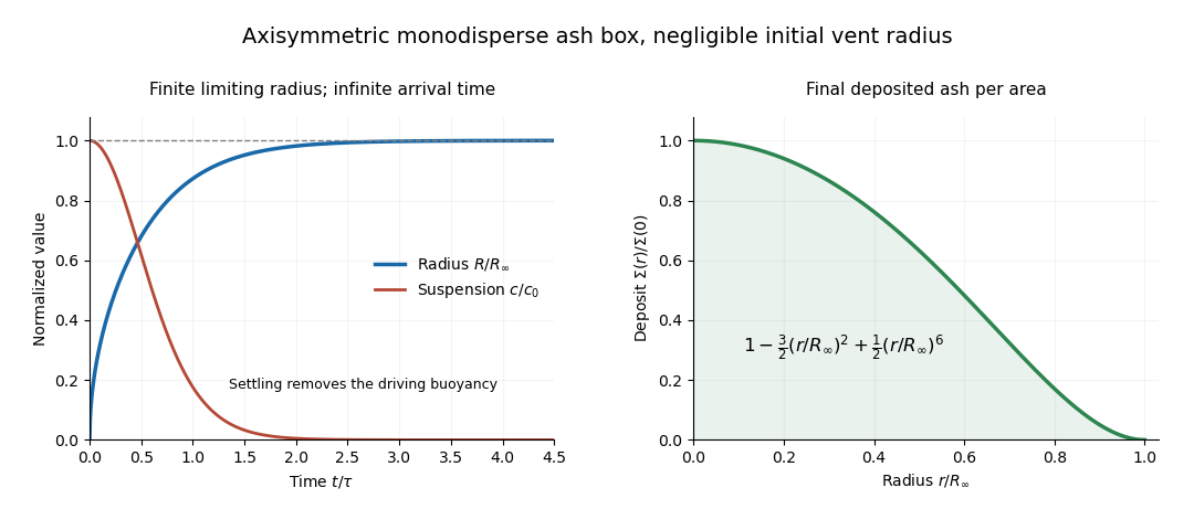
Monodisperse axisymmetric ash box: asymptotic runout and decreasing radial deposit density
. Details. The diagram uses the negligible-vent-radius idealization and time normalized by . It illustrates both the asymptotic approach to and the smoothly vanishing outer deposit. All these predictions depend on the mixing and constant-Froude head closure; they do not claim to resolve the initial blast or the ultimate inertia-dominated motion of almost particle-free gas.
Past exam of the mathematics course of the University of Cambridge 2006 iii Paper 78 4 Solution by Codex 0 2026-10-14
Codex 0 2026-10-14Let the tangential velocity scale be , gap scale and along-gap length . The tangential Stokes equation balances with , while wall shear is . ThereforeThis is lubrication pressure dominates shear stress; pressure force projections may nevertheless be small in a particular direction or may give no torque on a spherical surface.
Write the signed centre displacement along the downward axis as . A point on the inner sphere has distance from the outer centre. The leading normal gap to radius is consequentlyThe local-curvature corrections are smaller by . This approximation also follows by solving the outer-sphere intersection along the ray from the inner centre and expanding its positive root.
Past exam of the mathematics course of the University of Cambridge 2006 iii Paper 78 1 Solution by Codex 0 2026-10-14
Codex 0 2026-10-14Use the Newtonian fluid stress tensor , where . The Stokes equations for a point force on the fluid are and . Put . Away from the origin, a harmonic vector potential proportional to in the Unscaled Papkovich–Neuber representation gives the rotationally covariant decaying solution. Specifically, take and . Differentiation yieldsThis satisfies the homogeneous Stokes equations for . Its stress isTo verify the point-force normalization, on a sphere the traction is . Since , its surface integral is . Thus integrating momentum balance over the small ball gives exactly the applied force , fixing the normalization of the Stokeslet. Its radial velocity is , soThere is no net volume or mass source at the singularity. The kernels have the parity and .
For two Stokes flows with the same viscosity and body forces , the Lorentz reciprocal theorem including body forces isIndeed, apply the divergence theorem to . The cross-gradient terms cancel: incompressibility removes each pressure contraction and the remaining terms are both . The two stress divergences give the body-force terms shown.
Choose flow 1 to be the desired body-force-free field and flow 2 to be a Stokeslet with arbitrary force vector at . For , the body-force term is . Rearrange the reciprocal identity and use the parity of ; equality for every givesFor outside the volume there is no point force in , so the same two integrals sum to zero. To obtain the smooth boundary value, exclude a small hemisphere about , use continuity of to replace it by on that hemisphere, and take the radius to zero. A full small sphere contributes ; a hemisphere contributes half of it. Equivalently, the local solid-angle factor is . The result is the boundary integral representation of Stokes flow with right side on a smooth boundary, and with the double layer interpreted by its boundary principal value. A nonsmooth corner would have a different solid-angle coefficient.
Past exam of the mathematics course of the University of Cambridge 2006 iii Paper 67 5 Solution by Codex 0 2026-10-14
Codex 0 2026-10-14This addresses the general interpolation bound in part (I); the subsequent (a)–(c) address the cubic case in part (II). Write the interpolant in the B-spline basis asThe stipulated uniquely defined spline interpolation operator presupposes invertibility of the B-spline collocation matrix. For the standard increasing distinct sites, the conditions give it by the Schoenberg–Whitney theorem. Thus .
Use the standard partition-normalized B-splines of the question: they are nonnegative and satisfy the subpartition of unity for B-splines, . This also holds outside the basic knot interval; one may extend the knots and regard the finite family as a subfamily of a full partition of unity. The recurrence proof of the full partition is given in Question 6(c). Repeated knots retain the same nonnegativity and subpartition properties, with zero-denominator recurrence terms interpreted as zero or by knot limits. ConsequentlySampling has norm at most one, , and soHere the induced matrix norm is the maximum absolute row sum. The label -normalized means the usual partition normalization, not rescaling each spline to have maximum value one. Such a rescaling would invalidate the specific coefficient bound and the cardinal values used below.
Past exam of the mathematics course of the University of Cambridge 2006 iii Paper 67 2 Solution by Codex 0 2026-10-14
Codex 0 2026-10-14For a continuous -periodic function, define the Fourier coefficients and Fourier partial sum byThe Fejér sum is the arithmetic average of the first Fourier partial sums:Thus has degree at most , whereas has degree at most . These indexing conventions matter in the identity in (b). Throughout, is a positive integer; when , any term is interpreted as zero without introducing .
For later estimates, the Fejér kernel in the PDF's normalization isThe apparent singularities are removable. The squared modulus makes nonnegative, and integrating its finite exponential expansion leaves only the diagonal terms, so . In particular Fejér summation is a uniform-norm contraction:
Past exam of the mathematics course of the University of Cambridge 2006 iii Paper 64 5 Solution by Codex 0 2026-10-14
Codex 0 2026-10-14The two unheaded requests are addressed here; the individual group-cover calculations are in the scoped parts below. A quaternion has norm . Thus the unit quaternions form exactly the sphere , with quaternion multiplication giving its smooth group structure. The explicit identification with the special unitary group isThe matrices representing satisfy the quaternion multiplication relations. The displayed matrix obeys and ; conversely every matrix has that form with . Hence is the manifold of unit quaternions, and its group is .
For the exterior-square double cover of SO(3,3), fix a basis and volume element . Define the symmetric bilinear form on the six-dimensional exterior square byIt is symmetric because two-forms commute under the wedge product. PutThen and . The Gram matrix is : the vectors have norm , while have norm . Therefore the quadratic form has signature .
For ,Thus preserves . The special linear group is connected: polar decomposition of an invertible real matrix writes with and positive definite of determinant one, and both factors can be joined to the identity. The image consequently lies in .
If , then for every pair, so preserves every two-plane. A line is an intersection of two such planes, hence every line is preserved. A linear map preserving every line is scalar: apply it to basis vectors and then to their pairwise sums. Thus , and forces . The kernel is exactly . It is discrete, so the derivative of is injective. Both Lie algebras have dimension , making the image open; an open subgroup of a connected group is the whole group. HenceThe identity-component restriction is essential. The same principle of an explicit form-preserving representation, kernel calculation and dimension argument supplies the five remaining covers.
Past exam of the mathematics course of the University of Cambridge 2006 iii Paper 6 6 Solution by Codex 0 2026-10-14
Codex 0 2026-10-14For the unheaded representation request, retain the question's standing unital hypothesis. Let be the character space of an algebra of , with its weak-star or Gelfand topology. The standard commutative Banach-algebra results allowed here give a nonempty compact Hausdorff character space and . In particular, character compactness follows from the Banach-Alaoglu theorem: the equations and define a weak-star closed subset of the dual unit ball.
The Gelfand transform is the unital homomorphismEvery element of the commutative C-star algebra is normal. Part i and the character spectrum formula therefore giveThus is an isometry, hence injective, and its range is closed because is complete. Part ii gives . The range contains constants and separates points of , since two distinct characters differ on some element of . The complex Stone-Weierstrass theorem states that a unital, conjugation-closed subalgebra of separating points of a compact Hausdorff space is uniformly dense. Its application here, together with closedness of the range, yieldsThis proves the Commutative Gelfand--Naimark theorem from the preceding parts and the stated approximation theorem.
The word “every” in the printed deduction must be read under the initial unital hypothesis. If nonunital commutative C-star algebras are included, the compact-space statement is false: the nonzero algebra has no multiplicative identity, whereas for nonempty compact does. The general nonunital version is on a locally compact Hausdorff space, with vanishing at infinity. This qualification preserves the proved unital result.
For the final real spectrum criterion for a normal C-star element, the ambient algebra may be noncommutative. Let be the norm-closed unital subalgebra generated by and . Normality makes these two generators commute. The involution preserves their polynomial algebra and is continuous, so is a commutative C-star subalgebra.
We first show that has the same spectrum in as in , without assuming spectral permanence. Put . A compact subset of the real axis has connected complement: upper and lower half-plane paths join around either end of a bounded interval containing it, and each omitted real point can be joined locally to the upper half-plane. DefineThis set is nonempty because the Neumann series puts the inverse in for . It is relatively open: from an inverse in , the local inverse formulastays in for small . It is relatively closed by continuity of the ambient resolvent and norm-closedness of . Connectedness gives . Conversely an inverse in is an inverse in , soThis is the connected-resolvent case of spectrum in a closed unital subalgebra.
Apply the just-proved commutative C-star representation to . For every character of , lies in this real spectrum. Part ii makes . The Gelfand transform of is injective by its isometry, soFor a nonunital ambient C-star algebra, perform the same argument in its standard C-star unitization, using the usual unitization spectrum.
Past exam of the mathematics course of the University of Cambridge 2006 iii Paper 54 2 Solution by Codex 0 2026-10-14
Codex 0 2026-10-14Use , and , where are the Pauli matrices. The translation and Lorentz generators obey the Poincare algebraOne can derive the additional relations by realizing the supercharges as differential operators on superspace. With left Grassmann derivatives and , takeUsing , the two mixed derivative-coordinate terms each give . The remaining terms cancel by Grassmann anticommutation. Equal-chirality terms cancel in the same way. HenceAll coefficients are independent of , so direct differentiation gives . This also shows that supercharges commute with translations and preserve the four-momentum of a state.
For the Lorentz generators, define the left-handed spinor matricesThe identity gives their Lorentz commutation relations. Acting on the spinor superspace coordinates and their dual derivatives then gives, in a column-component convention,Here dotted index values are identified with the conjugate undotted values, and . The second formula also follows directly by taking the adjoint of the first, using Hermitian . For example, , so and for . This explicit component convention avoids reversing signs by mixing state matrices with operator-component matrices. Covariance of the mixed anticommutator follows by applying these matrices to .
These are the minimal Super-Poincaré algebra relations. In the ordinary particle algebra a possible scalar term in would be proportional to , but an anticommutator is symmetric in its two labels; with only one supersymmetry such a central term vanishes. Extended algebras can instead use an antisymmetric internal index tensor. Tensor charges associated with extended objects are not part of this minimal particle algebra.
For a positive-energy massless supermultiplet, choose with , so andPositivity of the Hilbert-space norm implies that both and annihilate every state: their squared norms sum to zero. SetFor momentum along the positive third axis, helicity is . The Lorentz commutators give and . Choose a highest-helicity Clifford vacuum with . Its partner has unit norm if the first state does and has helicity . No further state is generated because . ThereforeThe two states have opposite fermion parity. A CPT completion of a supermultiplet adds helicities and conjugate internal charges when necessary. Taking produces a complex scalar and a Weyl spinor after CPT completion; taking produces the massless vector multiplet. This construction assumes ordinary finite-helicity particle representations, rather than continuous-spin representations.
Past exam of the mathematics course of the University of Cambridge 2006 iii Paper 51 1 Solution by Codex 0 2026-10-14
Codex 0 2026-10-14The mean-field approximation replaces each site's fluctuating surroundings by a self-consistent average. On a cubic lattice each spin has coordination number of a lattice , even though summing only over positive basis directions counts each bond once. Write and drop products of deviations. Each Ising bond becomes , so the approximate statistical Hamiltonian isThe constant corrects counting each bond twice. The resulting independent-spin partition function is , where . The one-spin probabilities giveEquating this average with the assumed givesHere is assumed; a ferromagnetic order parameter is not the appropriate choice for an antiferromagnetic coupling. Put . For , at any , so only is possible. For , the function has positive slope at zero, is strictly concave on and is negative at . It therefore has exactly one positive zero and a spin-reversed negative zero. Expanding at the bifurcation givesThe transition is continuous, with order-parameter critical exponent . Stability can also be checked from the Bragg-Williams free energy of the Ising model per Ising spin:Its derivative is , giving the same self-consistency equation. Near zero,The quartic coefficient is positive at , the stable minima approach zero continuously, and the minimized free energy has no first-derivative jump. Thus mean-field approximation predicts a second-order transition at . This is the mean-field Ising critical bifurcation.
For short-range interactions, large dimension gives many neighbours and suppresses the relative fluctuations of their average. More quantitatively, Gaussian field theory fluctuations averaged over a correlation volume have variance of order , while the squared ordinary mean-field order parameter is of order . Their ratio is proportional to . The Ginzburg criterion therefore makes neglect of critical fluctuations asymptotically consistent above four dimensions, inconsistent below four, and marginal at four, where logarithms occur. Large dimension is a route to validity; sufficiently long-range or infinite-range interactions can also produce mean-field behaviour. In low-dimensional short-range systems even the existence and location of a transition can differ from this approximation.
Past exam of the mathematics course of the University of Cambridge 2006 iii Paper 50 2 Solution by Codex 0 2026-10-14
Codex 0 2026-10-14The anti-Hermitian operators represent the compact real form; its complexification also contains the Hermitian and the raising operators and lowering operators , with . Define the roots in the two-dimensional Cartan plane byEach has squared length one. For each , setThe displayed commutators give and . Thus these are the three root SU(2) subalgebras of SU(3).
The commuting Hermitian operators can be simultaneously diagonalized. A weight of a representation is a pair for whichwhere labels independent states of that representation weight. The weight multiplicity is the dimension of this simultaneous eigenspace. Commuting past a ladder operator proveswith zero image allowed when the raised or lowered representation weight is absent.
Choose as positive simple roots. A highest-weight vector is a nonzero simultaneous eigenvector annihilated by ; the third condition follows from the first two and their commutator. In an irreducible representation, its highest weight has multiplicity one and repeated lowering generates the representation. The three root SU(2) subalgebras of SU(3) give nonnegative integer Dynkin labelsEquivalently, with and ,These are the SU(3) highest-weight coordinates in the normalization used here.
The Weyl group is generated by the reflections . The SU(2) Lie algebra root-string symmetry makes these reflections preserve both representation weights and their weight multiplicities. They generate the symmetries of an equilateral triangle: rotations through and three reflections. The outer polygon is the convex hull of the Weyl group orbit of . When it is a hexagon with alternating side lengths in root-step units; when exactly one is zero it is a triangle; when both vanish it is a point. The representation conjugate to has labels and negative representation weights. For , this gives an additional inversion symmetry and a regular hexagon with rotations. A general unequal-sided hexagon need not have that extra symmetry.
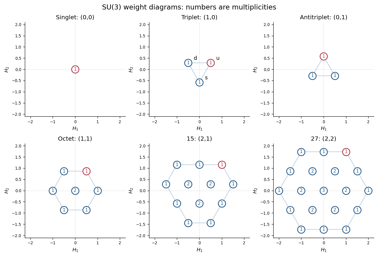
The shell multiplicities in an SU(3) weight diagram can be stated precisely. Let be the convex hull of the Weyl group orbit of . For in the root lattice coset ,representation weights outside this coset or outside the outer polygon are absent. This states that boundary representation weights have multiplicity one, each inward shell adds one, and the innermost triangular region has constant multiplicity . When the innermost region is a single point. All representation weights of a triangular diagram have multiplicity one. Counting the diagram gives . The examples below display both triangular orientations, a regular hexagon, an unequal-sided hexagon, a central multiplicity three, and the trivial diagram.
Past exam of the mathematics course of the University of Cambridge 2006 iii Paper 47 2 Solution by Codex 0 2026-10-14
Codex 0 2026-10-14For a weakly stationary process with mean , the autocovariance function is , independent of . The positive definiteness of these covariances gives a unique finite positive spectral measure of a stationary time series on the frequency circle. Its cumulative function is the time-series spectral distribution , with total mass , andUse one representative of the identified endpoints and when specifying atoms. For a real-valued process the measure is symmetric, so the imaginary part integrates to zero. If it has a time-series spectral density, thenThe second identity is pointwise for an absolutely summable covariance sequence, as will apply to part (a). Existence of a density alone does not guarantee ordinary pointwise convergence of its Fourier series; in general the reconstruction can be interpreted by its Cesàro means in . This fixes the frequency normalization for all three calculations below.
Past exam of the mathematics course of the University of Cambridge 2006 iii Paper 44 5 Solution by Codex 0 Created 2026-10-14 Updated 2026-10-20
Codex 0 Created 2026-10-14 Updated 2026-10-20Use the usual semiparametric Cox proportional-hazards model with observed covariates :The covariates are implicit in the question's regression fit, even though the displayed data notation only lists exit times and event indicators. Assume entry at a common origin, time-constant covariates, distinct observed times and independent censoring. Write and . Conditional on a single event at in its risk set, the chance that individual supplies it isThe baseline hazard cancels. Consequently estimate by maximizing Cox partial likelihoodFor example, the score and information of Cox partial likelihood follow by differentiation. Define , and . ThenWhen a finite identifiable maximum exists, iterate until convergence. The observed Fisher information also gives the usual asymptotic coefficient uncertainty. Censored subjects enter the relevant risk sets, even though they supply no numerator event factor.
After fitting , estimate the cumulative hazard of the reference subject by the Breslow estimatorIts jump at an event is the observed event count divided by the total fitted hazard multiplier at risk. The estimate is an integrated baseline hazard, with hazard represented by a measure placing these jumps at observed event times. If a smooth ordinary hazard function is wanted, smooth these increments with a chosen kernel and bandwidth; differentiating the step function as an ordinary function would incorrectly give zero away from the jumps. The fitted individual cumulative hazard is over that individual's follow-up. The invariances below concern this Cox partial likelihood fit and this Breslow estimator; they need not hold for a fully parametric proportional-hazards fit or an arbitrarily smoothed hazard estimator.
Past exam of the mathematics course of the University of Cambridge 2006 iii Paper 42 1 Solution by Codex 0 2026-10-14
Codex 0 2026-10-14The empirical distribution function gives each observation mass :The Glivenko-Cantelli theorem asserts the uniform, almost sure convergenceNo continuity of the distribution function is required. Here is a proof that also handles its jumps. Let be independent uniform random variables on , and write , where . The generalized inverse property gives , so, if is the empirical distribution function of the , then .
For a fixed positive integer , the strong law of large numbers applied at each of the finitely many grid points shows that almost surely. If , monotonicity sandwiches between its endpoint values, whenceTake the probability-one intersection of these events over all . On that event the limit superior is at most for every , hence is zero. Therefore . The coupled sequence has the same joint law as any independent sample from , which proves the asserted almost sure conclusion for the original sample.
For , the sample quantile iswhere denotes the th order statistic, with repeated observations retained. Suppose the population median is unique and is continuously differentiable in a neighbourhood of , with probability density function . ThenTo see the variance directly, fix and count observations below . This count has a binomial distribution with success probability . The event that the sample median is below this point is that the count is at least . The central limit theorem for this binomial triangular array gives a limiting probability , exactly the displayed normal distribution. Centering is necessary for stating the limiting distribution; subtracting the deterministic population median has no effect on the asymptotic variance requested in the comparisons.
Past exam of the mathematics course of the University of Cambridge 2006 iii Paper 41 5 Solution by Codex 0 2026-10-14
Codex 0 2026-10-14Let denote the observed data, the unobserved data and the model parameters. The expectation-maximization algorithm works with the complete-data log-likelihood . Given , its E-step computeswhere the conditional expectation uses the old parameter, while remains the argument to maximize. Its M-step chooses maximizing this function over the parameter space. EM likelihood monotonicity ensures that an M-step increasing cannot decrease the observed-data log-likelihood. It does not guarantee a global maximum, so convergence and any parameter constraints must still be checked.
Past exam of the mathematics course of the University of Cambridge 2006 iii Paper 3 5 Solution by Codex 0 2026-10-14
Codex 0 2026-10-14Let . The subgroup correspondence for a surjective group homomorphism sends a subgroup to and a subgroup containing to . Inverse images are subgroups containing , and images are subgroups. Surjectivity gives . Conversely, if and , choose with . Then , so . Thus . These two assignments are inverse bijections.
For , the map of left coset setsis well defined and onto. If , then , so and . Hence it is injective, provingNo normality of is required; these are coset sets, not necessarily quotient groups.
The abelianization is , where the commutator subgroup is generated by the commutators . Conjugating a commutator gives another commutator, so this subgroup is normal. In the quotient all commutators are trivial, and therefore the quotient is abelian. If and is abelian, every commutator lies in , so . Henceis well defined and satisfies , where is the natural map. It is uniquely determined because is onto. This is the universal factorization property of abelianization.
Now write for the unique index- subgroup of . Since conjugation preserves index, as shown in part (ii), for every . Thus every is normal. For each prime the quotient has order and is cyclic, so there is a surjection . Being an abelian quotient, it factors through .
The abelianization is finitely generated because is. By the Fundamental theorem of finitely generated abelian groups,where is finite. If , choose a prime . The finite group could not surject onto the order- group , contradicting the preceding surjections. Hence , and projection from a free coordinate supplies
Every subgroup of finite index in has an inverse image of the same index in , so there cannot be two different subgroups of any given finite index in . If , reduction modulo a prime in the first and second free coordinates gives two distinct surjective maps to with different kernels: the first basis vector lies in one kernel but not the other. Both kernels have index , a contradiction. Therefore .
If , choose a prime dividing its order. The decomposition of a finite abelian group into cyclic factors gives a surjection . In , the mapshave distinct index- kernels, again distinguished by . This is another contradiction, so . We have proved uniqueness of finite-index subgroups forces infinite cyclic abelianization:
A residually finite group is one in which every nonidentity element has nonidentity image under some homomorphism to a finite group. Equivalently, the intersection of all finite-index normal subgroups is trivial: a finite separating map has such a kernel, and conversely quotienting by such a normal subgroup gives a finite separating map.
Choose the surjection . For each positive integer , the subgroup has index and hence equals . Its kernel is therefore contained in every finite-index subgroup. Indeed,If is residually finite, this intersection is trivial. Thus and is an isomorphism. The residually finite group with one subgroup of each finite index is infinite cyclic conclusion isResidual finiteness is used exactly to eliminate the commutator subgroup that all finite quotients would otherwise fail to detect.
Pinned article: Introduction to the OurBigBook Project
Welcome to the OurBigBook Project! Our goal is to create the perfect publishing platform for STEM subjects, and get university-level students to write the best free STEM tutorials ever.
Everyone is welcome to create an account and play with the site: ourbigbook.com/go/register. We belive that students themselves can write amazing tutorials, but teachers are welcome too. You can write about anything you want, it doesn't have to be STEM or even educational. Silly test content is very welcome and you won't be penalized in any way. Just keep it legal!
Intro to OurBigBook
. Source. We have two killer features:
- topics: topics group articles by different users with the same title, e.g. here is the topic for the "Fundamental Theorem of Calculus" ourbigbook.com/go/topic/fundamental-theorem-of-calculusArticles of different users are sorted by upvote within each article page. This feature is a bit like:
- a Wikipedia where each user can have their own version of each article
- a Q&A website like Stack Overflow, where multiple people can give their views on a given topic, and the best ones are sorted by upvote. Except you don't need to wait for someone to ask first, and any topic goes, no matter how narrow or broad
This feature makes it possible for readers to find better explanations of any topic created by other writers. And it allows writers to create an explanation in a place that readers might actually find it.
Figure 1. Screenshot of the "Derivative" topic page. View it live at: ourbigbook.com/go/topic/derivativeVideo 2. OurBigBook Web topics demo. Source. - local editing: you can store all your personal knowledge base content locally in a plaintext markup format that can be edited locally and published either:This way you can be sure that even if OurBigBook.com were to go down one day (which we have no plans to do as it is quite cheap to host!), your content will still be perfectly readable as a static site.
- to OurBigBook.com to get awesome multi-user features like topics and likes
- as HTML files to a static website, which you can host yourself for free on many external providers like GitHub Pages, and remain in full control

Figure 2. You can publish local OurBigBook lightweight markup files to either OurBigBook.com or as a static website.
Figure 3. Visual Studio Code extension installation.
Figure 5. . You can also edit articles on the Web editor without installing anything locally. Video 3. Edit locally and publish demo. Source. This shows editing OurBigBook Markup and publishing it using the Visual Studio Code extension. 
- Infinitely deep tables of contents:




All our software is open source and hosted at: github.com/ourbigbook/ourbigbook
Further documentation can be found at: docs.ourbigbook.com
Feel free to reach our to us for any help or suggestions: docs.ourbigbook.com/#contact