Substitute the nonzero product $V=f(S)g(t)$ into the Black-Scholes equation with continuous stock dividends and divide by $fg$ on intervals where it is nonzero. The result isThe left side depends only on time and the right side only on spot, so both equal a constant $\lambda$. ThusThese are the separated solutions of the Black-Scholes equation. The zero solution is included separately, so division loses no relevant case.

For the unheaded parity request, the terminal difference of the power-call and power-put payoffs is $S_T^{\beta }-K^{\beta }$. Under the risk-neutral measure, $S_T=S\exp [(r-q-{\sigma }^2/2)\tau +\sigma (W_T-W_t)]$, where $\tau =T-t$. The Gaussian exponential moment gives ${\mathbb{E}}_Q[S_T^{\beta }\mid S_t=S]=S^{\beta }{e}^{{\lambda }_{\beta }\tau }$ with ${\lambda }_{\beta }=\beta (r-q)+{\sigma }^2\beta (\beta -1)/2$. Discounting the difference proves power put-call parity:For $\beta =1$ this is the familiar dividend-adjusted put-call parity, $S{e}^{-q\tau }-K{e}^{-r\tau }$.

The formula makes species the categorical response and the dot denotes all four other columns as candidate predictors. The classification tree is grown by recursive binary partitioning, not by fitting a linear regression to numerical species codes. At a node $t$, count observations of each class, $n_{tk}$, and set ${\hat{p}}_{tk}=n_{tk}/n_t$. These are the multinomial maximum-likelihood probabilities. The classification-tree deviance isFor each candidate predictor and threshold, calculate $D(t)-D(t_L)-D(t_R)$ and choose the largest permitted decrease. Continue recursively until a node is pure or the stopping controls prevent another split, for example because it has too few observations or insufficient deviance to warrant further growth. Only petal length, petal width and sepal length appear in the selected splits; sepal width was available but did not win a split. This greedy construction need not find a globally optimal tree. The default deviance criterion and recursive partitioning are documented in the tree package manual.

Each node number encodes its position: node $j$ has left and right children $2j$ and $2j+1$. The reported sample size is the number reaching the node; its deviance is calculated from that node's class counts. The fitted class is the class with largest fitted probability, with a convention resolving ties. The root's three counts are equal, so its displayed class is only a tie choice. An asterisk marks a terminal node, where prediction stops.

The resulting rule is displayed below. A left edge satisfies the stated strict inequality and a right edge its complement. None of the recorded training values lies exactly at these midpoint thresholds; the diagram adopts the right branch at equality for prediction.

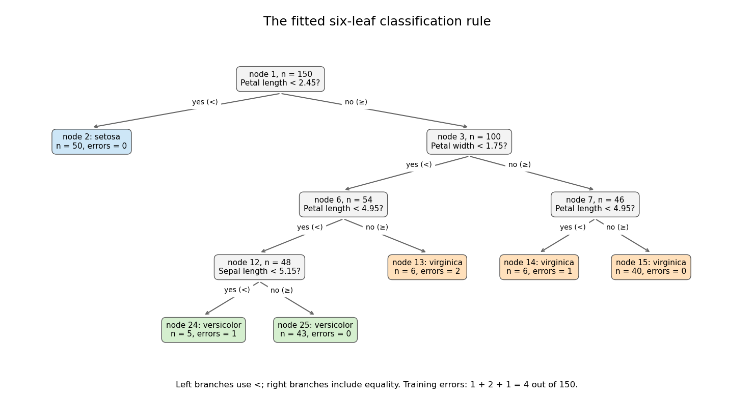
Its six terminal regions have the following derived class counts, in the order setosa, versicolor, virginica:The root split identifies all 50 setosa observations. Among the remaining specimens, the petal-width split is the principal separation of versicolor from virginica; further petal-length and sepal-length splits refine it. The leaf errors add to $4/150\simeq 2.67\%$. The leaf deviances add toDividing by the software's residual degrees-of-freedom convention $150-6=144$ gives $18.0489/144\simeq 0.1253$, as reported. The root deviance is $-2(150)\log (1/3)=300\log 3\simeq 329.6$. The deviance is a likelihood measure, whereas the error rate counts wrong majority-class predictions; these are different fit summaries.

Both quantities are in-sample, so the low error does not establish prediction accuracy on new specimens. Cost-complexity tree pruning, with tree size chosen by cross-validation, can remove weak splits and reduce overfitting. An independent test set is needed for a final estimate of the selected tree's prediction error.

For the sample, put $\bar{x}=n^{-1}{\sum }_i{x}_i$ and use the sample covariance matrixOrder its eigenvalues ${\hat{\lambda }}_j$ decreasingly and choose unit orthogonal eigenvectors ${\hat{\ell }}_j$. The sample principal components are the score columnsTheir sample means are zero and their sample covariance is diagonal, since ${\hat{\ell }}_j^{T}S{\hat{\ell }}_k={\hat{\lambda }}_j{1}_{\{j=k\}}$. The $j$th sample variance is ${\hat{\lambda }}_j$, and its explained variance of a principal component is ${\hat{\lambda }}_j/\mathrm{tr}(S)$. Using divisor $n$ instead changes the numerical variances by a common factor but leaves the component directions unchanged.

Standardizing means replacing a variable with positive sample variance by $(x_{ij}-{\bar{x}}_j)/s_j$. This gives principal component analysis on a correlation matrix, using $C=D^{-1/2}S{D}^{-1/2}$ with $D=\mathrm{diag}(S)$. It removes arbitrary differences of measurement units and prevents a large-variance coordinate from dominating solely through its scale. It also changes the question being optimized: small-variance and possibly noisy coordinates receive equal marginal weight. Principal component analysis based on the covariance matrix can be more appropriate when the variables have common meaningful units and absolute variability matters. Standardization is therefore a substantive choice, not an automatic improvement. A zero-variance variable must first be removed. In the word-rating example the variables share the same numerical range, but their across-word dispersions can differ; standardization gives each attribute equal initial variance.

For the standardized eight-variable analysis, total variance is $\mathrm{tr}(C)=8$. The first three fractions of explained variance of a principal component are approximately 59.6%, 19.1% and 10.1%, respectively. The first two account for about 78.8%, and the first three for 88.9%. The first direction is dominant but one direction alone loses substantial variation. Retaining two principal components is a plausible descriptive summary: their eigenvalues exceed $1$, whereas the third is below $1$. That cutoff is a heuristic, and the third principal component may still have interpretable content.

The reported coefficient rows are not unit-length vectors. The printed rounded rows have squared lengths $4.7514$, $1.5222$ and $0.8063$, consistent with their eigenvalues to the precision of the coefficient table. They are consistent with the scaled principal component loading convention $r_j=\sqrt{{\lambda }_j}{\ell }_j$. Such rows remain eigenvectors, but the score direction with unit length is ${\ell }_j=r_j/\sqrt{{\lambda }_j}$, or more accurately the row divided by its actual Euclidean norm when using rounded entries. Under this convention $r_{ij}$ is the correlation of standardized attribute $i$ with the variance-one score for component $j$:This explains both their sizes and why they must not be treated as the unit vectors from parts (i) and (ii).

The first principal component has positive coefficients on every attribute, strongest on friendliness, goodness, niceness, bravery and strength. With the favorable endpoints coded in the positive direction, it describes a broad favorable or impressive evaluation, with a potency contribution. The second contrasts movement and speed, with some size and strength, against the first three evaluative attributes; it is chiefly an activity dimension. The third is dominated by size, with smaller positive strength and negative movement/speed coefficients, distinguishing size or potency from activity. These are interpretations of directions of variation, not evidence of causal latent traits. Reversing a principal component's overall sign changes neither its meaning as an axis nor its explained variance; endpoint coding fixes only how its positive side is described.

Write the partitioned mean as $({\mu }_1^T,{\mu }_2^T{)}^T$ and assume $V_{22}$ is nonsingular, as required by the displayed inverse. For the conditional multivariate normal distribution, form the residualA linear transformation of a multivariate normal distribution is again normal. Direct calculation givesThe jointly normal blocks $U$ and $X_2$ are therefore independent: their joint characteristic function has no cross term in its quadratic exponent and factors into the two marginal characteristic functions. Conditioning leaves the distribution of $U$ unchanged. Reconstructing $X_1$ proves the full conditional law, including the requested Schur complement covariance:This describes a regular conditional law; it does not require the equality event to have positive probability.

A credibility estimate combines a risk's observed experience with collective or prior information, typically as $Z\overline{X}+(1-Z)m_0$. The credibility factor $Z\in [0,1]$ is the weight assigned to the individual experience: more reliable or more extensive data generally increases it. Bayesian credibility treats the risk parameter as random with a prior distribution and predicts future claims by averaging the conditional claim mean under its posterior distribution. Under squared-error loss this posterior predictive mean is optimal. It need not be an affine combination in every Bayesian model; the Poisson-gamma conjugacy calculation below yields that credibility form exactly, rather than as a best-linear approximation.

A scalar M-estimator is a selected root of $n^{-1}{\sum }_i\psi (Y_i,\hat{\theta })=0$, or equivalently a minimizer of a differentiable empirical objective whose derivative is this estimating equation. Its population statistical functional $T(F)={\theta }_F$ solves $\int \psi (x,{\theta }_F)dF(x)=0$. Assume local uniqueness, consistency of the sample root, a valid differentiable local expansion, finite ${\mathbb{E}}_F{\psi }^2$, andThese conditions include domination sufficient to differentiate under the integral and the required local uniform control of the sample derivative.

For $F_{\epsilon }=(1-\epsilon )F+\epsilon {\delta }_z$, differentiate the population estimating equation at $\epsilon =0$. Since its uncontaminated integral is zero,Thus the influence function is $\mathrm{IF}(z;T,F)=-\psi (z,{\theta }_F)/A$, with a proportionality constant independent of $z$.

Expanding the sample equation at its population root givesThe summands have mean zero. The central limit theorem and Slutsky's theorem therefore yield the scalar sandwich variance of an M-estimatorThis $V$ is the limiting variance of the $\sqrt{n}$-scaled error; the estimator's variance is approximately $V/n$. In a correctly centred location family with $\psi (x,\theta )=\psi (x-\theta )$, let $m={\mathbb{E}}_F{\psi }^{\prime }(X-\theta )$. Then $A=-m$, so the influence function is $\psi (z-\theta )/m$ and $V=\mathbb{E}{\psi }^2/m^2$. The minus sign from differentiating $x-\theta$ is essential.

The clipped Huber score in the subsequent subparts requires $0<b<\infty$. The PDF only displays an upper bound: at $b=0$ the estimating function vanishes identically, and at $b<0$ it is a constant with no root. A positive clipping threshold is the regular interpretation.

Write $a$ for the scalar intercept denoted $\mu$ in the question, to distinguish it from the individual means ${\mu }_i$. The log-likelihood of the independent Poisson observations isDifferentiating gives the score equations for an interior maximum-likelihood estimator:In particular, when $m={\sum }_i{y}_i>0$,The left side is a weighted covariate mean whose derivative is its weighted variance, so it is strictly increasing when the covariates are not all equal. An interior solution is unique if the observed count-weighted mean is strictly between the smallest and largest covariates. At an extreme it may require a limiting slope, and if all counts are zero the maximum occurs as $a\to -\infty$, rather than at finite parameters. Constant covariates make the slope and intercept unidentifiable.

Put $S_j={\sum }_i{x}_i^j{\mu }_i$. The negative Hessian matrix is deterministic at given parameters and is also the Fisher information matrix:Under the usual interior, increasing-information regularity for asymptotic normality of a maximum likelihood estimator, replace the unknown means by their fitted values and read the lower-right entry:Equivalently, Poisson slope information after eliminating an intercept is ${\sum }_i{\mu }_i(x_i-{\bar{x}}_{\mu }{)}^2$, with ${\bar{x}}_{\mu }=S_1/S_0$. This explains both the positive denominator for varying covariates and the loss of slope information when their spread is small.

Use the natural partial orderThe paper's shorthand $x\le x+y$ specifies the join order: more formally, $x\le z$ means $z=x+y$ for some $y$, which is equivalent to the displayed condition by idempotence. Associativity, commutativity and idempotence make addition the join operation. Distributivity makes multiplication monotone, while absorption gives $xy\le x$ and $xy\le y$.

Let $g_1,\dots ,g_r$ generate the incline. Distributivity writes every element as a nonempty finite join of monomialsThere is no assumed multiplicative identity: an exponent zero means omit that factor, and at least one factor remains. If $u\le v$ coordinatewise, absorption gives $m(v)\le m(u)$. If the two vectors are equal the conclusion is immediate; otherwise multiply $m(u)$ by the additional factors and apply absorption. For a polynomial with finite exponent support $A$, put $U_A=\{v:(\exists u\in A)u\le v\}$, its upward closure. If $U_A\supseteq U_B$, every monomial in $B$ is below some monomial in $A$, and consequently the join represented by $B$ is below the join represented by $A$.

We prove the reverse-inclusion well-quasi-ordering of monomial ideals, often called Maclagan's theorem, in the equivalent form that upward-closed subsets of ${\mathbb{N}}^r$ are well-quasi-ordered by reverse inclusion. Include the empty subset. For $r=1$, these are the tails $[n,\infty )$ and the empty set, corresponding to $\mathbb{N}\cup \{\infty \}$ in its usual well-order.

Induct on $r$. For an upward-closed $U\subseteq {\mathbb{N}}^r$, its slices $U_k=\{v\in {\mathbb{N}}^{r-1}:(v,k)\in U\}$ increase with $k$. Their union is upward closed and has finitely many minimal elements by the Dickson lemma; all those elements have appeared by some finite slice. Thus the slices eventually stabilize. Encode $U$ by the finite word of its pre-stabilization slices and its final stable slice. By the induction hypothesis, the slice order given by reverse inclusion is a well-quasi-ordering. The Higman lemma and finite product closure of well-quasi-orderings make these word-and-tail encodings well-quasi-ordered.

For a good pair of encodings $U,V$, an increasing subsequence map $f$ satisfies $U_k\supseteq V_{f(k)}$ at every pre-stabilization position of $U$, and the final slice of $U$ contains the final slice of $V$. Since $f(k)\ge k$ and the $V$ slices increase, $U_k\supseteq V_k$ before stabilization. Afterwards the final-slice comparison also gives $U_k\supseteq V_k$. Hence $U\supseteq V$, proving the induction. The use of Higman lemma is essential: finite-subset reverse domination does not preserve an arbitrary well-quasi-order, as the Rado order shows.

Given any infinite sequence of incline elements, choose a finite monomial support $A_i$ for each. The result just proved gives $i<j$ with $U_{A_i}\supseteq U_{A_j}$, hence $x_i\ge x_j$. Every finitely generated incline is therefore well-quasi-ordered by its reversed natural order.

We first prove invariance, before using any assertion that requires it. Write $A_n\phi (x)=n^{-1}{\sum }_{k=0}^{n-1}\phi (f^{k}x)$. Choose a point whose forward orbit has the prescribed convergence against every continuous function; the hypothesis gives a set of such points of full measure. For each continuous function $\phi$, telescoping givesbecause a continuous function on a compact metric space is bounded. Both test functions are continuous, so their averages converge to their prescribed integrals. Hencefor every continuous function $\phi$. The continuous-test criterion for an invariant measure therefore gives $f_{\ast }\mu =\mu$. The points in the hypothesis can now be called generic points for an invariant measure.

For ergodicity, let $B$ be a Borel set invariant modulo null sets, and set $h=1_B$, $p=\mu (B)$. Then $h\circ f=h$ almost everywhere. Since invariance preserves null preimages, deleting the union of all iterated preimages of the exceptional null set gives $h(f^{k}x)=h(x)$ for every $k\ge 0$ on one full-measure set. Thus $A_{n}h=h$ almost everywhere for every $n$.

Given $ϵ>0$, the continuous approximation of Borel indicators on a compact metric space, proved in the supporting steps below, supplies $\phi \in C(X)$ with $0\le \phi \le 1$ and $\Vert h-\phi {\Vert }_{L^1(\mu )}<ϵ$. By the hypothesis, $A_n\phi \to \int \phi d\mu$ almost everywhere. Since $0\le A_n\phi \le 1$, the dominated convergence theorem also gives convergence in $L^1(\mu )$. Invariance and the triangle inequality give the uniform estimateConsequently,Letting $n\to \infty$ and then $ϵ\downarrow 0$ proves $\Vert h-p{\Vert }_1=0$. Explicitly,so $p\in \{0,1\}$. Every invariant Borel set has measure zero or one, which provesThis proof controls measurable-set averages through a uniform $L^1$ estimate; convergence only against continuous test functions is not silently assumed to include indicator functions.