Topics (384k) Articles (398k) Users (410) Discussions (242) Comments (383) Files (13k) New article
A locally integrable function has weak derivatives on an open set exactly when it has them near every point. Local derivatives agree almost everywhere on overlaps because they define the same distributional derivative. A countable local cover therefore gives globally defined, locally integrable derivative functions. A smooth partition of unity subordinate to the cover splits each compactly supported test function; summing the local integration identities yields the global weak-derivative identity.
Bounded isolated-point removability for weak first derivatives by  Codex 0 Created 2026-10-14 Updated 2026-10-31
A bounded function which is away from one point in dimension , and whose classical gradient is locally integrable across that point, has that gradient as its weak derivative. Cut a test function off within distance of the point. The error from differentiating the cutoff is bounded by and vanishes. The other terms converge by local integrability. In dimension one the Heaviside step function is a counterexample: its classical derivative off the point is zero, but its distributional derivative is a Dirac delta.
If converges weakly to in a Banach space, there are convex combinations of each tail that converge in norm to .
The nonnegative Lp space functions have norm one. Any weak limit tested against indicators supported outside the origin must vanish almost everywhere. Testing against the constant bounded function one would nevertheless require integral one. This contradiction applies to every subnet whose indices tend to infinity, so the unit ball is not weakly compact. The abstract Banach-Alaoglu theorem remains valid: weak compactness of the unit ball is a different assertion from weak-star compactness of a dual ball.
In spatial sampling of a wave, a detector records a wave at positions separated by pitch . Angular wavenumbers differing by , with integers , give identical samples of a complex Fourier mode:This is spatial aliasing. To distinguish arbitrary sinusoids within a prescribed band, require , equivalently , the Nyquist spatial frequency. Thus for the shortest allowed wavelength. At equality a sine can vanish at every sample, so phase information can be lost. The Nyquist–Shannon sampling theorem states the precise reconstruction conditions for a bandlimited function; a finite scan introduces further limitations.
The synthetic two-tone snapshot iswhere both count cycles per metre. The component wavelengths are and . With , both lie below the Nyquist spatial frequency of cycles per metre. With , the -cycle component aliases to the -cycle component: at every , . The sampled sum is therefore indistinguishable from , although the continuous curves differ between samples. Drawing lines between sample points cannot resolve this ambiguity.
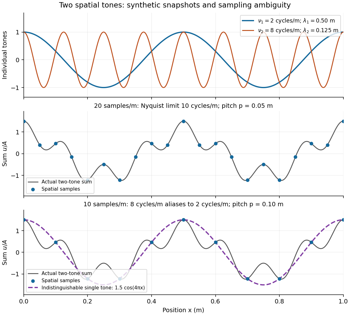
Synthetic two-tone spatial waveform: fine samples distinguish the components, coarse samples hide the shorter wavelength
. Details. A spectroscopic wavenumber commonly means the reciprocal of the vacuum wavelength of electromagnetic radiation, often in . It is an ordinary spatial frequency, so the vacuum angular wavenumber is . Specify vacuum or in-medium wavelength: the same frequency can have different wavelengths in different media. IUPAC's “wavenumber in medium” entry defines the in-medium reciprocal and notes that unqualified spectroscopic usage often means the vacuum reciprocal.[ref]
For example, a vacuum wavelength of corresponds to . Multiplication by gives . Converting centimetres to metres and converting cycles to radians are separate operations.
For a propagating branch of an ideal vacuum-filled rectangular electromagnetic waveguide, the phase velocity tracks constant wave phase along the axis, whereas the group velocity describes a sufficiently narrow, weakly distorted wave packet. Using givesThus , , and . Differentiating the dispersion relation proves the second formula; dividing it by proves the first. This is the same mathematical structure as Klein-Gordon packet velocities. In the stipulated example,Over , the corresponding narrow-envelope delay is , approximately . Timing a carrier wave crest would give ; it does not time the arrival of a newly introduced message.
There is an independent energy check. For the forward fields, the average axial Poynting vector is . Integrating across the guide gives average power and average electromagnetic energy per unit length :The transverse sine and cosine squared each integrate to ; then makes the integrated electric and magnetic contributions to equal. The axial energy transport therefore agrees with the group velocity in this ideal model.
As , and ; exactly at cutoff is undefined. Strong wave dispersion close to cutoff also limits the narrow-packet approximation. Neither a large phase velocity nor a pulse peak establishes superluminal information velocity; front velocity asks a separate causal question. In a uniform filling with constant positive permittivity and magnetic permeability , replace by , giving . Frequency-dependent material response or significant loss requires differentiating the actual dispersion relation, so this product is not universal.
Consider two identical two-segment paths from an inlet to a distal junction, with equal resistive beds at the two intermediate junctions and the distal junction. The segment transfer matrix and junction flow balances determine all pressures. If one inlet branch is removed and the beds are weakly loading the waves, the remaining segments form a three-segment chain with an effectively closed far end. The altered reflection pattern can raise peripheral oscillatory flow amplitudes even though a branch was lost; the incident wave amplitude, rather than total inlet pressure or flow, is the prescribed forcing.
Slowness is the reciprocal of phase velocity, measured in time per distance. A plane wave with wavevector and angular frequency has vector slowness . Its direction is the wavefront normal, which need not be the group velocity direction in an anisotropic medium.
The experiment in A time of flight method to measure the speed of sound using a stereo sound card by Carlos C. Carvalho and others makes wave speed visible as a delay. Two powered microphones feed separate channels of one stereo line input. A clap beyond one end of their common axis reaches the nearer microphone first. The displayed signals show two separated onsets when enlarged; count their sample separation to obtain and infer speed of sound from the measured microphone spacing . The reported sampling rate is . Repeating at different spacings gives a distance-versus-delay plot whose slope estimates speed of sound; dependence on distance helps identify acoustic travel rather than a fixed electronic delay. These are the paper's apparatus and observed readout, not measurements made for this article.[ref]
A controlled implementation also needs timing calibration for acoustic speed measurements. Put the microphones side by side to estimate the channel-delay offset , swap channels to check its sign, and check the acquisition clock against an independent timing reference. Measure spacings between consistent points on the microphones, keep the source outside their span and on their axis, and fit by linear regression rather than forcing a zero intercept. Repeat pulses and compare the same onset criterion before reflections arrive. These are proposed calibration and control checks, not additional procedures claimed for the paper.
One sample corresponds to for the reported sampling rate, so a delay of only a few samples has large relative measurement error. Background measurement noise, different microphone responses and threshold choice can move the apparent onset; reflections can supply a later competing pulse. Record temperature, keep air motion small, and compare several spacings. The result estimates speed of sound under those conditions; it cannot prove an exactly zero precursor below the instrument's sensitivity or establish finite propagation speed for every real medium. Both new diagrams in these sections show explicitly synthetic ideal wave equation solutions.[ref]
A fixed-end string of length initially straight receives velocity on an interval of width centred at , and zero elsewhere. Its sine-mode velocity coefficient is . For linear density , orthogonality gives mode energy and total energy . Their ratio is the displayed formula. Zeros in either sine factor suppress a normal mode completely.
For , the wave equation with zero endpoint displacement, zero initial displacement and initial velocity has the distributional weak solutionExpand the Dirac delta in the Fourier sine basis and solve each modal ordinary differential equation. Equivalently take the odd, -periodic extension of the initial velocity and use . The image impulses enforce the fixed endpoints. At jump fronts the Fourier series selects the midpoint of the two one-sided values.
Represent disconnected frazil ice and pancake ice as an upper layer with effective density, thickness and viscosity, rather than a continuous elastic plate. Linear Navier-Stokes equations in that layer are coupled to underlying water through velocity and stress conditions. A complex wavenumber describes both dispersion and wave attenuation in sea ice. A simpler conservative limit keeps ice mass loading but removes the elastic bending term; it does not predict viscous attenuation. The suspension model's effective viscosity is a fitted property, and a compact pancake cover need not behave like dilute frazil.
The wavevector times wave action gives the canonical momentum associated with translations of a wave's phase. It describes momentum exchange with a slowly varying mean fluid flow, rather than simply the spatial average of oscillating fluid momentum. For horizontal wavenumber , its horizontal component is . A convention using displacement pseudomomentum of an internal gravity wave instead has the opposite sign.
Define the proper electromagnetic vertex with the electric charge removed, and define without the propagator's overall factor . The displayed off-shell identity follows by localizing the vector symmetry in a time-ordered correlation function, including the contact terms at the charged-field insertions, and amputating. Its on-shell form gives the Ward identity for physical photon amplitudes. At zero photon momentum it identifies the vertex with the momentum derivative of the inverse fermion propagator.
For tree electron-Positron annihilation into three photons, all six orders along the fermion line must be summed. Write and . Contracting an internal photon with its momentum gives when . Contracting an end photon removes its adjacent Dirac propagator by the external Dirac equation, with a minus sign at the electron end and a plus sign at the positron end. For either fixed order of the two uncontracted photons, the three insertion positions therefore telescope to zero. Summing their two orders proves the Ward identity. The mass terms in both remaining Dirac propagators are essential when . The result expresses the invariance of the scattering amplitude under .
The dimensionless ratio of a medium's permittivity to vacuum permittivity. The constant scalar value used in a Wannier-Mott exciton is an approximation to the relevant material response.
For , the Wang sequence and the mapping degree of the antipodal map give . If is odd, ; if is even, and . All other groups vanish. At the mapping torus is a torus with . At , the two-point swapping mapping torus is a circle. Every example is already a closed manifold; for it is orientable exactly when is odd.
For inviscid planar incompressible flow, write velocity as and vorticity as . Taking curl of the Euler equations for an inviscid fluid removes pressure and gives the displayed transport equation, with . The Poisson equation then recovers the streamfunction at each instant. A velocity tangent to the plane cannot stretch its perpendicular vorticity vector.
Nonrotating layerwise-two-dimensional vortex dynamics by Codex 0 Created 2026-10-14 Updated 2026-10-18
Codex 0 Created 2026-10-14 Updated 2026-10-18In the limiting model of infinitely strong stable density stratification, small Froude number and fixed vertical scales suppress vertical displacement. Each horizontal level evolves by two-dimensional vortex dynamics; labels independent copies of the horizontal Poisson equation. The leading normalized Ertel potential vorticity is . This is a constrained asymptotic model: finite buoyancy frequency restores vertical motion and coupling, and arbitrarily short vertical scales invalidate the independent-layer limit. McIntyre's discussion of potential-vorticity inversion explains the limiting independent-layer picture.
Pinned article: Introduction to the OurBigBook Project
Welcome to the OurBigBook Project! Our goal is to create the perfect publishing platform for STEM subjects, and get university-level students to write the best free STEM tutorials ever.
Everyone is welcome to create an account and play with the site: ourbigbook.com/go/register. We belive that students themselves can write amazing tutorials, but teachers are welcome too. You can write about anything you want, it doesn't have to be STEM or even educational. Silly test content is very welcome and you won't be penalized in any way. Just keep it legal!
Intro to OurBigBook
. Source. We have two killer features:
- topics: topics group articles by different users with the same title, e.g. here is the topic for the "Fundamental Theorem of Calculus" ourbigbook.com/go/topic/fundamental-theorem-of-calculusArticles of different users are sorted by upvote within each article page. This feature is a bit like:
- a Wikipedia where each user can have their own version of each article
- a Q&A website like Stack Overflow, where multiple people can give their views on a given topic, and the best ones are sorted by upvote. Except you don't need to wait for someone to ask first, and any topic goes, no matter how narrow or broad
This feature makes it possible for readers to find better explanations of any topic created by other writers. And it allows writers to create an explanation in a place that readers might actually find it.
Figure 1. Screenshot of the "Derivative" topic page. View it live at: ourbigbook.com/go/topic/derivativeVideo 2. OurBigBook Web topics demo. Source. - local editing: you can store all your personal knowledge base content locally in a plaintext markup format that can be edited locally and published either:This way you can be sure that even if OurBigBook.com were to go down one day (which we have no plans to do as it is quite cheap to host!), your content will still be perfectly readable as a static site.
- to OurBigBook.com to get awesome multi-user features like topics and likes
- as HTML files to a static website, which you can host yourself for free on many external providers like GitHub Pages, and remain in full control

Figure 2. You can publish local OurBigBook lightweight markup files to either OurBigBook.com or as a static website.
Figure 3. Visual Studio Code extension installation.
Figure 5. . You can also edit articles on the Web editor without installing anything locally. Video 3. Edit locally and publish demo. Source. This shows editing OurBigBook Markup and publishing it using the Visual Studio Code extension. 
- Infinitely deep tables of contents:



All our software is open source and hosted at: github.com/ourbigbook/ourbigbook
Further documentation can be found at: docs.ourbigbook.com
Feel free to reach our to us for any help or suggestions: docs.ourbigbook.com/#contact