For $1<\mu \le \sqrt{2}$, the interval $J=[1/(\mu +1),\mu /(\mu +1)]$ is invariant under the second iterate of the tent map. The affine coordinate $h(x)=(\mu /(\mu +1)-x)/((\mu -1)/(\mu +1))$ conjugates that restriction to the tent map with parameter ${\mu }^2$. Its two linear pieces give the identity directly. This turns the two-iterate horseshoe threshold into a four-iterate threshold and explains why chaotic invariant sets need not have periodic points near the original nonzero fixed point.

Restrict $T_s(x)=1-s|x|$ to $[-1,1]$, with $1<s\le 2$. Its image is the closed intervalBecause $0\in A$ and ${\max }_{x\in A}|x|=1$, its next image is again $T_s(A)=A$. Every state in $[-1,1]$ therefore enters this invariant core after at most one iterate and remains there. This is the core used in interval exactness of a tent-map core.

The domain restriction matters. If the same formula defines a map on the whole real line, any $x<-1/(s-1)$ stays on the negative branch and satisfiesThus points outside the declared phase interval need not enter $A$, and $A$ is not a globally absorbing interval for the real-line extension.

For a short exact sequence $0\to U\stackrel{i}{\to }V\stackrel{q}{\to }W\to 0$ and any module $E$, the sequence $U{\otimes }_{A}E\to V{\otimes }_{A}E\to W{\otimes }_{A}E\to 0$ is exact. The last map is surjective since every pure tensor $w\otimes e$ can be lifted using a preimage of $w$. Put $T=(V{\otimes }_{A}E)/\mathrm{im}(i\otimes 1_E)$. There is a well-defined balanced map $W\times E\to T$, sending $(q(v),e)$ to the class of $v\otimes e$: replacing $v$ by $v+i(u)$ changes it by an element of the discarded image. This induces $W{\otimes }_{A}E\to T$, inverse to the map induced by $q\otimes 1_E$. Thus the kernel of $q\otimes 1_E$ is exactly the image of $i\otimes 1_E$. Consequently a module is flat exactly when tensoring with it also preserves injections.

Identify the product with endomorphisms of the defining space. Special unitary group conjugation fixes scalar matrices and preserves the complementary traceless subspace. For $N\ge 2$, the latter is the complex Adjoint representation of a Lie algebra, which is irreducible because ${\mathfrak{sl}}_N$ is simple. With fundamental Dynkin index $1/2$, the trace-Casimir identity gives $C_2(\mathbf{N})=(N^2-1)/(2N)$; the tensor-product Casimir trace identity then gives $C_2(\mathbf{Adj})=N$.

For a $G$-representation $V$ and an $H$-representation $W$ over the same field, $V⊠W$ is the representation of $G\times H$ on $V\otimes W$ given by $(g,h)(v\otimes w)=gv\otimes hw$. Its character is $(g,h)\mapsto {\chi }_V(g){\chi }_W(h)$. For finite groups $G,H$, over a splitting field for finite group representations in characteristic zero the external products of irreducible representations form all irreducible representations of $G\times H$: character orthogonality gives irreducibility, and their squared degrees sum to $|G||H|$, proving exhaustion. Unlike the tensor product of two representations of one group, the two factors here act independently.

The two-factor tensor rank is the smallest number of pure tensors whose sum equals $t$, with zero allowed as the empty sum. For two finite-dimensional vector spaces over the same field, it equals the matrix rank of the tensor-product coefficient matrix. A sum of $r$ outer products has column space contained in the span of their $r$ first factors, so its matrix rank is at most $r$. Conversely, choose a basis $u_1,\dots ,u_r$ for the column space, express each column in that basis, and collect the coefficients into row vectors $w_k^T$. This yields $C={\sum }_{k=1}^r{u}_k{w}_k^T$, hence a sum of $r$ pure tensors.

The pure tensor $(2,1)\otimes (-1,3)$ therefore has two-factor tensor rank one, whereas $e_1\otimes f_1+e_2\otimes f_2$ has two-factor tensor rank two. Both have two factors: the number of factors and the minimum number of product summands are different counts. Over the real numbers, the singular value decomposition supplies a useful decomposition $C={\sum }_k{\sigma }_k{u}_k{v}_k^T$, with one nonzero term per matrix rank. The two-factor rank equality does not extend to three or more factors by merely choosing one matrix layout.

In a two-factor tensor product over a field, a pure tensor is also called a separable or decomposable tensor: it can be expressed as one product $v\otimes w$. Every tensor is a finite sum of pure tensors, but a sum need not itself be a pure tensor.^[ref]

For finite-dimensional vector spaces, the tensor-product coefficient matrix gives a decisive test: a nonzero tensor is a pure tensor exactly when its matrix rank is one. Indeed, every column of $v{w}^T$ is a scalar multiple of $v$. Conversely, if all columns of a nonzero matrix are multiples of one nonzero column $v$, collect their multipliers in $w$ to obtain $C=v{w}^T$. The zero tensor is also a pure tensor, for example $0\otimes w$, but its matrix rank is zero.

In ${\mathbb{R}}^2{\otimes }_{\mathbb{R}}{\mathbb{R}}^2$, the tensoris nonseparable: its matrix rank is two and its determinant is one, whereas $\det (v{w}^T)=0$. Directly, trying $t=(a{e}_1+b{e}_2)\otimes (c{f}_1+d{f}_2)$ requires $ac=bd=1$ and $ad=bc=0$. The first two equations force all four scalars nonzero, contradicting the others. In contrast, products sharing a factor do combine: $e_1\otimes f_1+e_1\otimes f_2=e_1\otimes (f_1+f_2)$. Thus being written as two summands alone does not establish nonseparability.

An antisymmetric tensor changes sign under exchange of two indices in a specified subset of its indices. A totally antisymmetric tensor has this property for every pair of indices.

Symmetrization over $r$ selected tensor indices is the average over all $r!$ permutations, with every sign positive. Parentheses denote this operation, for example $T_{(ab)}=(T_{ab}+T_{ba})/2$. It is a projection onto the symmetric part and commutes with a covariant derivative acting on indices outside the parentheses.

Antisymmetrization over selected tensor indices averages their permutations with the sign of a permutation. Square brackets denote it, for example $T_{[ab]}=(T_{ab}-T_{ba})/2$. It projects onto the alternating part. Antisymmetrized second derivatives of a scalar vanish for a torsion-free connection, but antisymmetrized later derivatives act on a tensor and can produce curvature.

The Lagrangian integral time is the area under a normalized velocity autocorrelation along a Lagrangian trajectory. If this correlation is integrable, Taylor turbulent dispersion has asymptotic mean-square displacement $2R_L(0)t_{L}t$. The integral time need not equal every short-time decorrelation scale, particularly when the autocorrelation oscillates.

For stationary statistics along a Lagrangian trajectory $\mathbf{X}$, the velocity autocorrelation depends on the lag $s$. Integrating velocity twice gives the mean-square displacement $2{\int }_0^t(t-s)R_L(s)ds$. If $R_L$ is integrable, the long-time displacement is diffusive. Its normalized one-sided area is the Lagrangian integral time.

For a zero-mean stationary velocity process of variance ${\sigma }_v^2$ and normalized autocorrelation $(1+|s|{)}^{-\alpha }$, integrating velocity twice gives the displayed expression, exactly rather than just asymptotically. For $\alpha >1$ the long-time diffusion coefficient is ${\sigma }_v^2/(\alpha -1)$. At $\alpha =1$, the displacement variance is asymptotic to $2{\sigma }_v^{2}t\log t$. For $0<\alpha <1$, it is asymptotic to $2{\sigma }_v^2{t}^{2-\alpha }/[(1-\alpha )(2-\alpha )]$. Linear variance growth does not by itself imply a central limit theorem or a normal distribution for displacement.

For a smooth real function satisfying the displayed equation with positive integer $r$, differentiating makes $f^{(j+r)}=f^{(j)}$. On any compact interval, all derivatives are therefore bounded by the maximum of the bounds of $f,f^{\prime },\dots ,f^{(r-1)}$. The Taylor formula with integral remainder consequently has error at most $M{R}^{n+1}/(n+1)!$, which tends to zero uniformly for $|x|\le R$. Hence the function equals its globally convergent Taylor series. For $r=3$ and initial derivatives $(1,0,0)$, it is ${\sum }_{k\ge 0}{x}^{3k}/(3k)!$.

In nearly columnar flow between rigid boundaries, a geostrophic contour is a contour of column height divided by the Coriolis parameter. If relative vorticity is negligible, conservation of shallow-water potential vorticity constrains leading geostrophic flow to these contours. Motion across them stretches or squashes columns, generating relative vorticity; for constant $f$, the contours are simply contours of $H$.

Let $G$ be cyclic and let $R[G]$ carry the regular permutation action. Invariants are constant coefficient vectors, which are the images of the norm operator. A vector with coefficient sum zero is the difference of a vector and its cyclic translate, by successively solving the coordinate differences. Thus the norm group kernel equals $(\sigma -1)R[G]$. Both cyclic Tate cohomology groups vanish. This applies to $R=\mathbb{Z}$ and $R={\mathbb{Z}}_p$, and to finite direct sums of regular lattices.

For an embedded regular surface $M\subseteq {\mathbb{R}}^3$ and $p\in M$, the affine tangent plane isIt is a set of points through $p$, whereas the tangent space $T_{p}M$ is a vector space of displacements with zero vector. Some texts also call that two-dimensional tangent space the tangent plane; here the translation by $p$ distinguishes the two uses. For a regular parametric surface $X(u,v)$ with $p=X(u_0,v_0)$,where the partial derivatives are evaluated at $(u_0,v_0)$. Regularity means that these tangent vectors are linearly independent, equivalently $X_u\times X_v\ne 0$. Their cross product is a normal vector. ^[ref]

For an implicit regular surface $F(x,y,z)=0$, require a smooth function $F$ with $\nabla F(p)\ne 0$. ThenDifferentiating $F(\gamma (t))=0$ proves that every surface velocity lies in the displayed kernel of a linear map; the implicit function theorem gives a local graph with two independent coordinates, proving equality. The gradient is the normal vector with respect to the ambient dot product. ^[ref]

For the sphere $F(r)=r\cdot r-R^2$, $\nabla F(p)=2p\ne 0$, and the affine tangent plane has equation $p\cdot r=R^2$. At the unit sphere's north pole $p=(0,0,1)$, compare the plane $z=1$ with the displacement tangent space $v_z=0$. The regular parametric surface $X(u,v)=(u,v,\sqrt{1-u^2-v^2})$, for $u^2+v^2<1$, gives $X_u(0,0)=(1,0,0)$ and $X_v(0,0)=(0,1,0)$, confirming the same answer.

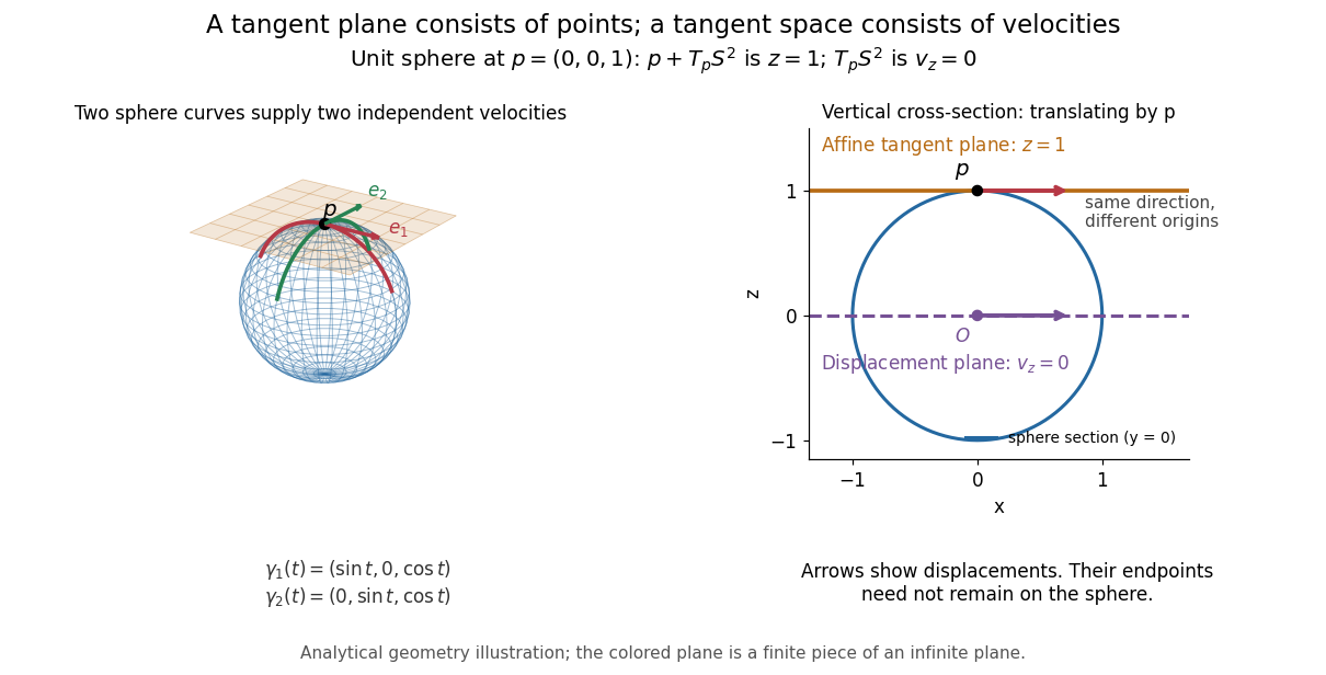
This analytical illustration shows a unit sphere and a vertical cross-section. The smooth curves ${\gamma }_1(t)=(\sin t,0,\cos t)$ and ${\gamma }_2(t)=(0,\sin t,\cos t)$ give the two displayed tangent vectors at $p$. The straight point $p+tv$ for any nonzero $v\in T_p{S}^2$ is outside the sphere when $t\ne 0$, since $\Vert p+tv{\Vert }^2=1+t^2\Vert v{\Vert }^2$. A tangent plane therefore captures first-order motion, not an exact patch of the regular surface.

The same idea makes local approximation useful. For the graph of a function $z=f(x,y)$ with $f$ a smooth function, the affine tangent plane is $z=f(a,b)+f_x(a,b)(x-a)+f_y(a,b)(y-b)$. ^[ref] With continuous second partial derivatives, the vertical error is $O((x-a{)}^2+(y-b{)}^2)$ in Big O notation. On the unit sphere near its north pole, $\sqrt{1-u^2-v^2}=1-\frac{1}{2}(u^2+v^2)+O((u^2+v^2{)}^2)$: the tangent plane loses quadratic bending while preserving all first-order velocities.

A failed regularity test needs interpretation. Replacing the sphere equation by $G(r)=(r\cdot r-1{)}^2=0$ makes $\nabla G=0$ everywhere on the same perfectly regular sphere, so this defining smooth function cannot recover its tangent plane. Similarly, the usual spherical parametric surface loses matrix rank at the poles, while the graph parametrization above remains regular there. A vanishing gradient or degenerate parametrization invalidates that calculation; it alone does not prove that the underlying geometry has no tangent plane.

For mutually independent random variables, every tail event has $\mathbb{P}(A)\in \{0,1\}$. Identical probability distributions are unnecessary. The tail sigma-algebra is trivial in probability: its events have probability zero or one, though it can contain nonempty proper sets.^[ref]

For a proof, set ${\mathcal{F}}_m=\sigma (X_1,\dots ,X_m)$ and ${\mathcal{F}}_X=\sigma (X_1,X_2,\dots )$. Independence extended from generating pi-systems makes ${\mathcal{F}}_m$ independent of $\sigma (X_{m+1},X_{m+2},\dots )$, hence of each tail event $A$. The increasing union ${\bigcup }_m{\mathcal{F}}_m$ is a generating pi-system for ${\mathcal{F}}_X$. For fixed $A$, the events $B$ satisfying $\mathbb{P}(A\cap B)=\mathbb{P}(A)\mathbb{P}(B)$ form a Dynkin system. The pi-lambda theorem extends this equality to all $B\in {\mathcal{F}}_X$. Taking $B=A$ givesThus $A$ is independent of itself, forcing the two stated values.^[ref]

The useful feature is the absence of intermediate probabilities for infinite properties that ignore every finite prefix. It reduces some calculations to showing that a tail event has positive probability, or that its complement does. The theorem supplies no finite observation deadline, and an extra argument such as the calculation in infinitely many heads as a tail event is needed to decide which value occurs.

On the full Cartesian product $\Omega ={\mathbb{R}}^{\mathbb{N}}$ with its product sigma-algebra, take the coordinate random variables $X_j(x)=x_j$. A product-measurable set $A$ is a tail event if and only if membership is unchanged whenever two sequences differ in finitely many coordinates. The measurability condition is essential: invariance alone is not a license to assign a probability to an arbitrary subset.

For the forward implication, fix $m$. An event in $\sigma (X_{m+1},X_{m+2},\dots )$ cannot distinguish points with the same remaining coordinates. Since a tail event belongs to this sigma-algebra for every $m$, every finite change preserves membership.

For the converse, freeze the first $m$ coordinates to zero. The insertion mapis a measurable function for the product sigma-algebras. Thus $B_m=i_m^{-1}(A)$ is a measurable set. Invariance gives $A={\pi }_m^{-1}(B_m)$, where the coordinate projection ${\pi }_m$ discards the first $m$ entries. Hence $A\in \sigma (X_{m+1},X_{m+2},\dots )$ for every $m$. The same argument works on $\{0,1{\}}^{\mathbb{N}}$. On a general probability space, coordinates need not admit arbitrary replacements, so the defining intersection of sigma-algebras remains the reliable formulation.

For a nonnegative random variable, $Y={\int }_0^{\infty }{1}_{\{Y>t\}}dt$ pointwise, including when $Y=\infty$. Tonelli's theorem permits taking expectation under the integral and proves the formula in the extended nonnegative reals. This relates finiteness of a Brownian exit time expectation to integrability of its survival probability.