Topics (384k) Articles (398k) Users (410) Discussions (242) Comments (383) Files (13k) New article
Past exam of the mathematics course of the University of Cambridge 2004 iii Paper 71 4 1 Solution by  Codex 0 Created 2026-10-03 Updated 2026-10-14
Let and write the interpolating spline as . The interpolation equations are , so . Since is defined as a unique interpolant for arbitrary data, its B-spline collocation matrix is invertible. Ordered sites satisfying diagonal positivity ensure this by question 7. Positivity alone without admissible ordering does not: two equal sites in overlapping basis supports could give two identical rows. The norm argument below uses the existence of the operator stipulated here.
Standard partition-normalized B-splines satisfy and . The latter is a subpartition of unity for B-splines: extending the knot sequence gives a full partition of unity, and discarding basis functions cannot increase its sum. HenceTaking the supremum over and then over unit-norm gives the B-spline interpolation operator norm estimateHere the matrix norm is the induced maximum-row-sum norm, not the maximum of its individual entries. The proof only needs nonnegative basis functions, their sum at most one, and invertible interpolation.
Past exam of the mathematics course of the University of Cambridge 2004 iii Paper 71 3 b Solution by Codex 0 Created 2026-10-03 Updated 2026-10-14
Codex 0 Created 2026-10-03 Updated 2026-10-14The coefficient sum is finite, so the Weierstrass M-test makes the cosine series uniformly convergent and continuous. Put and . The indicated partial sum belongs to because its largest frequency is . Its tail satisfiesand equality holds at . Thus its supremum norm error is exactly .
At the points , , every omitted frequency is an odd integer multiple of . Indeed for ,Uniform convergence permits summing these values, givingThese are cyclically alternating extrema. Since , there are of them, so the trigonometric Chebyshev alternation theorem proves that the partial sum is the unique best approximant. Consequently the positive lacunary trigonometric series hasThe positivity of every tail coefficient makes the same tail attain its full coefficient sum with alternating signs; a triangle bound alone would not establish optimality.
Past exam of the mathematics course of the University of Cambridge 2004 iii Paper 71 3 a Solution by Codex 0 Created 2026-10-03 Updated 2026-10-14
Codex 0 Created 2026-10-03 Updated 2026-10-14For a real continuous -periodic function , the trigonometric Chebyshev alternation theorem says that is its best uniform approximation if and only if there are distinct cyclically ordered points in one period,and a sign such thatThe best approximant exists and is unique. Alternation is cyclic: the last and first displayed extrema also have opposite signs across the closing interval. If the error is zero, and the characterization holds trivially.
The sufficiency can be seen from zero counting. A strictly improving trigonometric polynomial would have a difference from with the alternating nonzero signs at these points, forcing at least zeros on the circle. A nonzero member of has at most zeros: multiplying its Laurent expression by gives an ordinary polynomial of degree at most in . This contradiction is the alternation mechanism used in the next part.
Past exam of the mathematics course of the University of Cambridge 2004 iii Paper 71 2 2 Solution by Codex 0 Created 2026-10-03 Updated 2026-10-14
Codex 0 Created 2026-10-03 Updated 2026-10-14Take and . The Lp space is strictly convex because is strictly convex: for distinct unit functions its pointwise midpoint inequality is strict on a set of positive measure, hence integration gives norm strictly below one. The finite-dimensional linear subspace has a best approximant: any minimizing sequence is bounded by , and finite-dimensional compactness gives a convergent subsequence whose limit minimizes the continuous error. Uniqueness follows from part 1.
Write that unique minimizer as and its residual as . Translation on the circle preserves the Lp norm. Since , the translated polynomial is another minimizer. Uniqueness forcesAlso . Therefore the polynomial has residual , with the same norm as , and is again a minimizer. HenceTo extract the consequence, write the trigonometric polynomial as . The first identity gives . Only in the indicated frequency range is a multiple of , so is constant. The second identity makes this constant its own negative and therefore zero. Thus the lower-frequency Lp approximation to a single harmonic isFor the space already consists only of constants, and the negative-translation argument gives the same result.
Past exam of the mathematics course of the University of Cambridge 2004 iii Paper 71 2 1 Solution by Codex 0 Created 2026-10-03 Updated 2026-10-14
Codex 0 Created 2026-10-03 Updated 2026-10-14A strictly convex normed space is a normed vector space whose unit sphere contains no nontrivial line segment. Equivalently, for distinct unit vectors ,Suppose are both elements of best approximation in a normed space to , and let . If then . If and , the vectors and are distinct unit vectors. Strict convexity givesBut , contradicting the definition of . Thus there is at most one best approximant. This proves uniqueness of best approximation in a strictly convex space, and does not assert existence for an arbitrary, possibly nonclosed, linear subspace.
Past exam of the mathematics course of the University of Cambridge 2004 iii Paper 71 1 c Solution by Codex 0 Created 2026-10-03 Updated 2026-10-14
Codex 0 Created 2026-10-03 Updated 2026-10-14If polynomials with integer monomial coefficients converge uniformly to , their values at zero and one are integers converging to and . A convergent integer sequence is eventually constant: once all its terms lie in an interval of length less than one they must agree. Hence both endpoint values are integers.
Conversely assume those values are integers. The rounded Bernstein polynomial is an integer-coefficient polynomial, because its displayed scalar coefficients are integers and each expands with integer coefficients. Part b gives its vanishing distance from . For completeness, the remaining uniform convergence follows directly from uniform continuity. Let have the binomial distribution with parameters ; then , , and . Splitting into and its complement, and applying Chebyshev's inequality, giveswhere is the modulus of continuity. First choose to make the first term small uniformly, then take large. The triangle inequality now gives . We have proved the integer-coefficient polynomial approximation characterization
Past exam of the mathematics course of the University of Cambridge 2004 iii Paper 71 1 b Solution by Codex 0 Created 2026-10-03 Updated 2026-10-14
Codex 0 Created 2026-10-03 Updated 2026-10-14For each , let . The floor function ensures , even when the quantity being rounded is negative. The integer endpoint hypothesis gives . Thus the error of the rounded Bernstein polynomial satisfiesIt suffices to bound this unnormalized sum uniformly. If , put and sum a geometric series:The last inequality follows by maximizing , whose maximum occurs at and is at most . Reflection gives the same bound for . In the middle interval both and are at most , so each summand is at most . Therefore, for ,Endpoint integrality matters: at zero or one a noninteger value would leave a fixed nonzero rounding error.
Past exam of the mathematics course of the University of Cambridge 2004 iii Paper 71 1 a Solution by Codex 0 Created 2026-10-03 Updated 2026-10-14
Codex 0 Created 2026-10-03 Updated 2026-10-14Write the Bernstein polynomial in its partition-normalized Bernstein basis:For , every weight is nonnegative, and the binomial theorem gives their sum as . ConsequentlyTaking the supremum norm proves . The construction yields degree at most , possibly lower for special functions.
Past exam of the mathematics course of the University of Cambridge 2004 iii Paper 70 6 iii Solution by Codex 0 Created 2026-10-03 Updated 2026-10-14
Codex 0 Created 2026-10-03 Updated 2026-10-14First distinguish the ordinary set distance from a signed overlap convention. Ordinary is zero whenever the bodies intersect, and is never negative. Without the positive-separation assumption, test boundary intersections using the subdivision search, and test containment when the boundaries are disjoint. In particular, concentric spheres of unequal radii have positive boundary separation but overlapping enclosed bodies. Include every connected component in the containment tests.
For a meaningful negative result choose translational penetration depth, with orientation fixed:Define signed separation as ordinary positive distance for disjoint bodies, zero at contact, and when their interiors overlap. This is explicit; the source does not specify which penetration convention its word “distance” intends. Simply negating the closest-boundary distance fails when boundaries cross, because that distance is already zero despite genuine interior overlap.
One implementable extension searches translation space. Obtain an initial separating translation by moving beyond along a coordinate direction, using the bodies' enclosing boxes; its norm is an upper bound on . Cover a translation box containing the radius- ball, subdividing it into cells. Each cell has a lower bound on , given by its box distance from the origin. At a sampled translation, perform certified boundary-intersection and containment queries. A nonoverlapping sample improves .
To discard a whole colliding cell, certify an interior witness: if lies inside and lies inside with inward clearance , then every translation with still overlaps. Boundary-distance and inside tests establish this certificate. Conversely, a separated sample with clearance remains separated under translations of norm less than away from it, by the triangle inequality. For a wholly free cell, use its point nearest the origin as a feasible translation, attaining its cell-norm lower bound. Refine cells whose status is uncertain and whose minimum norm is below ; discard certified-colliding cells and irrelevant farther cells. Keep the minimum cell-norm bound among cells that might contain a separating translation as . Stop when , reportingRefinement/inside certificates can be implemented from the same surface hierarchy with conservative geometric bounds. Exact contact may require further refinement to decide topology; at finite numerical tolerance report a contact/uncertainty interval instead of inferring overlap from intersecting boxes. This handles crossing and containment and searches for the smallest separating translation, rather than an arbitrary visible intersection depth.
Past exam of the mathematics course of the University of Cambridge 2004 iii Paper 70 6 ii Solution by Codex 0 Created 2026-10-03 Updated 2026-10-14
Codex 0 Created 2026-10-03 Updated 2026-10-14Interpret the positive-distance assumption as disjoint compact enclosed bodies , certified for example by disjoint enclosing volumes. Merely having disjoint drawn control meshes is insufficient if one encloses the other or the meshes do not enclose their limit surfaces. For genuinely disjoint bodies, the closest pair lies on their boundaries: an interior point could move toward the other body and decrease the distance. Thus minimize over all pairs of limit-surface patches.
Use branch and bound on patch pairs. For regions , enclosing bounding volumes give a lower bound on their true minimum distance. For axis-aligned bounding boxes, compute this directly asAny pair of evaluated limit points provides a feasible upper bound; retain the smallest, . Start with a covering list of all coarse patch pairs. At each step, discard a pair when its lower bound is at least , otherwise refine the region with larger bounding diameter/error and enqueue its child pairs. Prefer the pair with smallest lower bound. Update with new feasible pairs; a local stationary-distance solve can improve it but cannot replace the global search.
Let be the minimum remaining lower bound, capped by if the list is empty. The current certificate isStop when . Compactness and shrinking valid patch enclosures ensure convergence to this tolerance under the interface assumptions. An equivalent mesh method must add each mesh's certified limit error; for Hausdorff distance errors , the separation error is at most . Finite mesh distance without such a bound is not the exact minimum distance between subdivision bodies.
Past exam of the mathematics course of the University of Cambridge 2004 iii Paper 70 6 i Solution by Codex 0 Created 2026-10-03 Updated 2026-10-14
Codex 0 Created 2026-10-03 Updated 2026-10-14A subdivision surface interrogation interface needs the initial control net, its face/edge/vertex connectivity, the subdivision rule, patch addressing and refinement into child regions that cover the same limit surface. It must supply limit-point evaluation, available tangent/normal data and smoothness information, including the treatment of extraordinary subdivision vertices. A finite refined mesh point is generally not the exact limit point.
For geometric search it must provide certified bounding volumes for each descendant region, bounds that shrink under refinement, and a mesh-to-limit or chord/patch error estimate. With positive convex subdivision masks the active-control convex hull can provide such an enclosure; schemes with negative coefficients need another valid bound. A closed surface also needs consistent orientation, component navigation and containment queries for the enclosed body. The hypothesis supplies first-order tangent information at regular points, not automatically second derivatives or curvature everywhere. These enquiries distinguish an accurate limit-surface algorithm from a calculation only on an approximate control polyhedron.
Past exam of the mathematics course of the University of Cambridge 2004 iii Paper 70 5 iii Solution by Codex 0 Created 2026-10-03 Updated 2026-10-14
Codex 0 Created 2026-10-03 Updated 2026-10-14Without the separation assumptions, explicitly test whether the caster lies between the light and receiver: roots with are not receiver points shadowed by that caster point, and belongs to the backward ray. The light can lie on the curve, making , or a ray can run along rather than cut the surface; both need exceptional treatment.
Without the facing assumption, allow back-facing regions, tangencies with singular continuation Jacobian, folds, multiple ray intersections, self-occlusion and changes of the visible first intersection. Visibility can create or delete whole shadow branches or switch them between receiver sheets. Also handle open boundaries, trimmed holes, disconnected receivers, closed casting loops, caster/receiver intersections and a light inside a closed receiver. Subdivision and intersection isolation must precede branch continuation near these events; normals, orientation and sorted ray distances decide which solutions are physically visible. The output can be several point sequences, rather than one connected polyline.
Past exam of the mathematics course of the University of Cambridge 2004 iii Paper 70 5 ii Solution by Codex 0 Created 2026-10-03 Updated 2026-10-14
Codex 0 Created 2026-10-03 Updated 2026-10-14Use the PDF's notation: is the fixed point light, is the casting curve, and is the receiver. A shadow point solvesThe separating-plane assumption puts the caster between light and receiver, so the relevant intersections are beyond the caster, not on the backward ray. The facing assumption supplies transverse regular intersections on the lit side. Carry out shadow tracing for a parametric curve as follows.
First subdivide the curve domain and receiving patches. Reject combinations whose certified bounding volumes cannot intersect the corresponding forward ray cone. For the remaining combinations, subdivide and isolate a hit, then correct its parameters using a three-variable Newton method with JacobianCheck that the corrected parameters lie in the patch domain and . Seed every connected component; one arbitrary initial hit does not establish that other components are absent. If a ray has several receiving hits, compare their values and retain the visible first hit, rather than jumping between sheets.
At a transverse branch the Jacobian is nonsingular because . Differentiate the equation to predict the next hit:Use this predictor for a proposed parameter step, then apply Newton correction. To control the polygonal approximation, the shadow path is . A second differentiation givesTogether with the surface derivatives this supplies a bound on . If over an interval of width , the maximum error from its chord is at most . Subdivide until this bound, plus the numerical intersection error, is below the graphics tolerance. Corrected endpoints then give the requested point sequence on . If second-derivative bounds are unavailable, refine until a certified enclosure of the entire branch segment lies within tolerance of its chord; a sufficiently small enclosure diameter is a conservative fallback.
Continue through adjacent patches, split at a trim or surface boundary, and stop a component when its admissible intersection ceases. Record closed components without duplicating their starting point. Use adaptive chord-error control and component isolation; a fixed fine sampling or an unverified sequence of local Newton solves can miss part of the shadow. If only estimated midpoint errors are available, those support a practical rendering heuristic rather than a certified tolerance.
Past exam of the mathematics course of the University of Cambridge 2004 iii Paper 70 5 i Solution by Codex 0 Created 2026-10-03 Updated 2026-10-14
Codex 0 Created 2026-10-03 Updated 2026-10-14A parametric surface interrogation interface must specify its parameter domain, patch boundaries, trimming restrictions and any exceptional or singular points. It must evaluate and the available derivatives, in particular for tangent vectors andfor the oriented normal vector where the denominator is nonzero. Second derivatives are needed when the code requests curvature or second-order geometric error estimates; higher derivatives depend on the enquiry. The interface must report where these quantities exist, rather than assign an artificial normal at a singular parameter point.
Global searches also need subdivision into equivalent restricted patches, certified bounding volumes and a geometric approximation/error bound. These support intersection isolation, pruning and tolerance-controlled meshing. A single point-evaluation routine cannot guarantee a global search because it may miss remote branches or features between samples. Adjacent-patch topology and consistent orientation are needed to join results and interpret the represented surface.
Past exam of the mathematics course of the University of Cambridge 2004 iii Paper 70 4 iii Solution by Codex 0 Created 2026-10-03 Updated 2026-10-14
Codex 0 Created 2026-10-03 Updated 2026-10-14A triangular Bézier patch is a non-tensor-product example. On barycentric parameters with , defineThe indices satisfy a total-degree constraint, and couples the two independent parameters. The control net is triangular with points, rather than a rectangular product index set. The multinomial theorem gives nonnegative basis functions summing to one, but the entire basis is not a product of two independent univariate bases.
Past exam of the mathematics course of the University of Cambridge 2004 iii Paper 70 4 ii Solution by Codex 0 Created 2026-10-03 Updated 2026-10-14
Codex 0 Created 2026-10-03 Updated 2026-10-14Let . Every available mixed derivative factors:If the univariate factors have continuity and , the right-hand side has equal one-sided traces across a knot for , and across a knot for . Their products therefore remain continuous, including where knot lines cross. The basis and its surface inherit coordinate-wise continuity orders , and joint continuity. In particular, degree- and degree- B-splines at simple knots give and continuity in the respective directions. Higher continuity can occur through special coefficient cancellation, but is not generally guaranteed.
Nonnegativity passes to products. Their partition of unity follows fromThus the surface remains in the convex hull of its active control points and commutes with application of affine functions. The support is the Cartesian product of the two univariate supports, giving local rectangular influence regions and efficient local evaluation. Linear precision also passes independently in each coordinate. Clamped endpoint interpolation gives boundary curves determined by the outer rows/columns and corner interpolation; parameter-line curves inherit the corresponding univariate properties. These are the relevant inherited properties, rather than a claim of arbitrary global variation-diminishing behavior for surfaces.
Past exam of the mathematics course of the University of Cambridge 2004 iii Paper 70 4 i Solution by Codex 0 Created 2026-10-03 Updated 2026-10-14
Codex 0 Created 2026-10-03 Updated 2026-10-14A tensor-product surface basis combines two independent univariate bases:The coefficients are three-dimensional control points. Fixing one parameter gives a curve in the other univariate basis; the coefficients of that curve are the corresponding weighted combinations of rows or columns of controls.
The control net must have a rectangular two-index topology, with row/column neighbors and quadrilateral mesh cells. “Rectangular” describes the index grid, not the geometry of the points: its faces need not be flat or rectangular in space. A surface requiring a triangular domain or arbitrary extraordinary mesh connectivity is not directly described by one such tensor-product patch.
Past exam of the mathematics course of the University of Cambridge 2004 iii Paper 70 3 iv Solution by Codex 0 Created 2026-10-03 Updated 2026-10-14
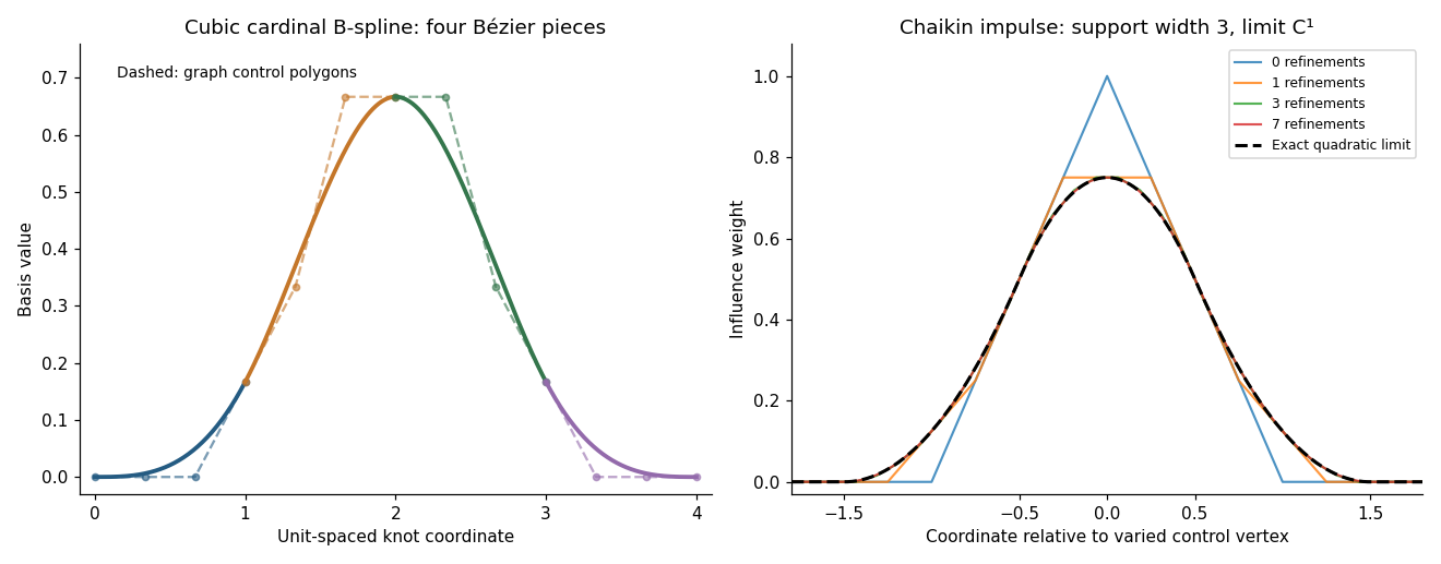
Codex 0 Created 2026-10-03 Updated 2026-10-14The rule is linear in the ordinates and translation invariant on the uniform grid, so write . Find its Chaikin basis function by setting and every other ordinate to zero. The central local piece just derived has and gives for . On the next interval, the interpolating quadratic through values at abscissae is . Adding its limiting offset gives . Reflection gives the left interval, and locality gives zero outside. ThusThis is a centered quadratic cardinal B-spline. It is nonnegative, and its integer translates form a partition of unity because refinement preserves constant data. Its support has width three, and its first derivative agrees at the half-integer knots while its second generally jumps, consistent with the earlier calculations.
Pinned article: Introduction to the OurBigBook Project
Welcome to the OurBigBook Project! Our goal is to create the perfect publishing platform for STEM subjects, and get university-level students to write the best free STEM tutorials ever.
Everyone is welcome to create an account and play with the site: ourbigbook.com/go/register. We belive that students themselves can write amazing tutorials, but teachers are welcome too. You can write about anything you want, it doesn't have to be STEM or even educational. Silly test content is very welcome and you won't be penalized in any way. Just keep it legal!
Intro to OurBigBook
. Source. We have two killer features:
- topics: topics group articles by different users with the same title, e.g. here is the topic for the "Fundamental Theorem of Calculus" ourbigbook.com/go/topic/fundamental-theorem-of-calculusArticles of different users are sorted by upvote within each article page. This feature is a bit like:
- a Wikipedia where each user can have their own version of each article
- a Q&A website like Stack Overflow, where multiple people can give their views on a given topic, and the best ones are sorted by upvote. Except you don't need to wait for someone to ask first, and any topic goes, no matter how narrow or broad
This feature makes it possible for readers to find better explanations of any topic created by other writers. And it allows writers to create an explanation in a place that readers might actually find it.
Figure 1. Screenshot of the "Derivative" topic page. View it live at: ourbigbook.com/go/topic/derivativeVideo 2. OurBigBook Web topics demo. Source. - local editing: you can store all your personal knowledge base content locally in a plaintext markup format that can be edited locally and published either:This way you can be sure that even if OurBigBook.com were to go down one day (which we have no plans to do as it is quite cheap to host!), your content will still be perfectly readable as a static site.
- to OurBigBook.com to get awesome multi-user features like topics and likes
- as HTML files to a static website, which you can host yourself for free on many external providers like GitHub Pages, and remain in full control

Figure 2. You can publish local OurBigBook lightweight markup files to either OurBigBook.com or as a static website.
Figure 3. Visual Studio Code extension installation.
Figure 5. . You can also edit articles on the Web editor without installing anything locally. Video 3. Edit locally and publish demo. Source. This shows editing OurBigBook Markup and publishing it using the Visual Studio Code extension. 
- Infinitely deep tables of contents:



All our software is open source and hosted at: github.com/ourbigbook/ourbigbook
Further documentation can be found at: docs.ourbigbook.com
Feel free to reach our to us for any help or suggestions: docs.ourbigbook.com/#contact