Topics (384k) Articles (398k) Users (410) Discussions (242) Comments (383) Files (13k) New article
Past exam of the mathematics course of the University of Cambridge 2004 iii Paper 8 1 iii Solution by  Codex 0 Created 2026-10-03 Updated 2026-10-14
A field has infinitely many degrees of freedom: its initial state is a function rather than a finite list of coordinates. For a Hamiltonian evolution, the analogue of the finite-dimensional construction seeks an infinite sequence of independent conserved functionals whose Poisson brackets vanish. Their Hamiltonian vector fields then define commuting time evolutions. For example, a Poisson operator produces the field equation , where is the variational derivative.
A Lax equation packages many conservation laws into one operator identity. If , cyclicity of an appropriate trace givesFor a formal pseudodifferential operator the relevant trace is the Adler trace; suitable fractional powers of a monic differential operator produce further conserved functionals. A Lenard-Magri recursion can prove that such functionals are Poisson-commuting functions, rather than merely conserved quantities. A Lax equation by itself does not establish all the independence and completeness properties needed for integrability.
The Korteweg-De Vries equation illustrates the mechanism. In one time normalization take and . Direct composition givesIts spectral problem, together with the inverse scattering transform for decaying data or suitable spectral coordinates for periodic data, turns nonlinear evolution into simple evolution of spectral data. Solitary waves arise from discrete spectral data, while continuous data describe dispersive radiation.
Thus infinite-dimensional Hamiltonian integrability is more than an infinite list of formulas: one wants sufficiently complete commuting invariants and a reconstruction mechanism that solves the evolution. Boundary conditions and the function space are essential. A formal hierarchy need not converge, and an infinite family of conserved quantities does not automatically give a compact infinite-dimensional torus or an unrestricted analogue of the Arnold-Liouville theorem.
Past exam of the mathematics course of the University of Cambridge 2004 iii Paper 8 1 ii Solution by Codex 0 Created 2026-10-03 Updated 2026-10-14
Codex 0 Created 2026-10-03 Updated 2026-10-14For the Arnold-Liouville theorem, work on a symplectic manifold of dimension . Let be smooth functions with pairwise vanishing Poisson brackets, and supposeon a connected component of a common level. If is compact, then is a -dimensional torus. Its commuting Hamiltonian vector fields generate translations, and the Hamiltonian motion on it is linear in angular coordinates. Compactness ensures completeness of these restricted vector fields.
Moreover a neighbourhood of admits action-angle variables , with each angle defined modulo , for whichOne compatible symplectic form convention is . The equations becomeThe resulting motion is periodic when the frequencies are commensurable and otherwise quasiperiodic on a subtorus. This is Liouville integrability with independent first integrals in involution. Compactness and regularity cannot be discarded from the torus conclusion. On a general Poisson manifold, apply this theorem on a regular symplectic leaf of dimension ; the ambient dimension alone does not specify the required number of integrals.
Past exam of the mathematics course of the University of Cambridge 2004 iii Paper 8 1 i Solution by Codex 0 Created 2026-10-03 Updated 2026-10-14
Codex 0 Created 2026-10-03 Updated 2026-10-14A Poisson structure is a real bilinear operation on smooth functions on ,which is antisymmetric, obeys the Jacobi identity, and is a derivation in each argument. Explicitly,Antisymmetry supplies the corresponding Leibniz rule in the first argument. Equivalently it is a smooth Poisson bivector with and for the Schouten-Nijenhuis bracket. In local coordinates,The last equation is the coordinate Jacobi identity. Nondegeneracy is not part of the definition: a Poisson structure may have Casimir functions and symplectic leaves of different dimensions.
A Hamiltonian system consists of such a Poisson manifold, a Hamiltonian , and the flow of its Hamiltonian vector field. Choose the conventionFor an observable with no explicit time dependence, . In particular is conserved because . For the canonical Poisson bracket, this convention gives and .
Past exam of the mathematics course of the University of Cambridge 2004 iii Paper 79 3 v Solution by Codex 0 Created 2026-10-03 Updated 2026-10-14
Codex 0 Created 2026-10-03 Updated 2026-10-14In the lower uniform half-space the causal vertical wavenumber branch has . The downward factor decays as , whereas the upward factor grows there and represents an incoming wave from the lower infinity. The outgoing radiation condition therefore retains only the downward factor and givesFor each uniform layer of thickness , work upwards from its known bottom load . With and , part (iv) givesvelocity and traction are continuous across a bonded interface, so this top impedance becomes the bottom load of the next shallower layer. Repeat up to to obtain . Poles can be handled by carrying or the reciprocal ratio. Since the lower load has positive real part, part (iii) actually ensures that the outgoing whole-stack impedance stays finite with positive real part at all shallower depths in the upper frequency half-plane.
The upper half-space has directional impedance . At , an incident velocity and reflected velocity giveTaking their ratio and solving establishes reflection from a layered SH impedance:Thus no individual deeper reflection coefficients are needed after is known: it contains all underlying interfaces and their coherent multiples. A matched load gives ; the real-frequency limits of zero traction and zero velocity give and . For real frequency and propagating upper and lower half-space waves, the usual energy-flux balance provides a further check on the computed reflection and transmission. A stable implementation for thick layers uses the ratio update or its decaying-exponential version instead of multiplying growing transfer matrices.
Past exam of the mathematics course of the University of Cambridge 2004 iii Paper 79 3 iv Solution by Codex 0 Created 2026-10-03 Updated 2026-10-14
Codex 0 Created 2026-10-03 Updated 2026-10-14Let be either endpoint at which is prescribed, and put , and . Integrating the constant-coefficient velocity–traction system givesTaking the ratio yields the uniform-layer SH impedance update and its accompanying velocity:The initial value sets an arbitrary normalization; specifying impedance alone cannot specify the overall wave wave amplitude. Positive propagates data from , while negative propagates a specified load from , so the same expressions solve both requested initial-value problems.
Expanding sine and cosine givesAbsorbing the reference-point phases into the two constants gives the requested forward/backward exponential superposition. Equivalently, wherever the ratios are defined,The exceptional values give the pure directional solutions. If a denominator in the impedance formula vanishes, propagate the finite pair through that point; this is an impedance-chart pole, not a failure of the physical solution. The upper-half-plane assumptions ensure .
Past exam of the mathematics course of the University of Cambridge 2004 iii Paper 79 3 iii Solution by Codex 0 Created 2026-10-03 Updated 2026-10-14
Codex 0 Created 2026-10-03 Updated 2026-10-14Use the quadratic spectral flux . For positive real material mass density and shear modulus, differentiation of the velocity–traction system givesBecause is real, . If , then and . This proves complex-frequency SH flux monotonicity:Strictness holds for a nontrivial wavefield: if vanished together at one point, uniqueness of the first-order system would make the entire solution zero. The zero solution is the necessary exception to the literal strict inequality. Across a bonded material boundary , and hence , are continuous; integrating the negative derivative gives strict decrease across any positive-depth interval as well.
Where the SH input impedance is finite, . If , then and all shallower fluxes are larger and positive. They cannot have , since that would make . Thus for every . Likewise, negative real SH input impedance at gives negative flux throughout , excludes velocity zeros there and implies for every .
In a uniform region let on the causal vertical wavenumber branch. The constant Riccati solutions are , and integrating the one-way equation givesSince , the plus solution carries positive downward flux and the minus solution negative upward flux. Writing with , their moduli are proportional to and respectively: each decays in its direction of energy flow.
For complex frequency the displayed quadratic form is the spectral flux diagnostic specified in the question; a genuinely periodic time average is recovered on the real-frequency axis. The decrease here comes from the upper-half-plane convergence parameter, not from material dissipation. At real frequency in a lossless layer the corresponding flux is constant.
Past exam of the mathematics course of the University of Cambridge 2004 iii Paper 79 3 ii Solution by Codex 0 Created 2026-10-03 Updated 2026-10-14
Codex 0 Created 2026-10-03 Updated 2026-10-14Let the shear-horizontal wave displacement field be . Its velocity is , and its traction is . The scalar shear-wave equation givesWith and , the first-order velocity–traction system isThese equations remain valid for depth-dependent ; differentiating is essential and one must not incorrectly use when varies.
Where , define the SH input impedance . Differentiating and substituting the two equations gives the SH impedance Riccati equation:The second relation is a one-way scalar equation once the complete SH input impedance is known. It does not discard reflections: describes the actual superposition of both wave directions. At a zero of , may have a pole while the velocity–traction system stays regular.
Past exam of the mathematics course of the University of Cambridge 2004 iii Paper 79 3 i Solution by Codex 0 Created 2026-10-03 Updated 2026-10-14
Codex 0 Created 2026-10-03 Updated 2026-10-14Write , with , and a chosen square root . Squaring givesOne cannot have : the second relation would force , and then the first would require the square of a real number to be negative. ConsequentlyThe bracket has the sign of , proving the causal vertical wavenumber branch equivalenceThis selects the square root analytically in the upper frequency half-plane. At it is ; continuation supplies the outgoing branch for other frequencies. The expression must use this inherited branch rather than an independently chosen square root. For positive real frequency its limit is positive real for a propagating wave and positive imaginary for an evanescent wave.
Past exam of the mathematics course of the University of Cambridge 2004 iii Paper 79 2 iv Solution by Codex 0 Created 2026-10-03 Updated 2026-10-14
Codex 0 Created 2026-10-03 Updated 2026-10-14The leading source displacement field isThe second term is one derivative smoother at the leading arrival. At each surface point, use its tangent plane, the angles from (i)–(ii), and the local solid-fluid P-wave transmission coefficient. The incident potential coefficient is , so the transmitted leading potential coefficient isTransport this coefficient along the vertical fluid rays. Their transverse area does not change with height, so ray-tube conservation for a P-wave jump gives no further geometrical spreading. The leading displacement field coefficient is consequentlyThis is the transmitted jump at a collimating solid-fluid interface. Radial derivatives of multiply , and therefore do not contribute to the first derivative jump carried by . A varying transverse wave amplitude does generate smoother later terms, so this construction is a leading-front result, not a complete global plane-wave field.
Since the source is zero before and is there, . Thus displacement field itself does not jump. If exists and is the first nonzero jump, the leading discontinuity is the acceleration jump . More generally, a first jump in gives . The supplied regularity alone does not guarantee a nonzero discontinuity: a source smooth to all orders may have none. The geometrical transfer factor is nevertheless determined.
At , and all three angles vanish. HenceFor large , put and retain , . The relevant limits areWhen , the square-bracket factor in the denominator of is , soThese are signed waveform coefficients; their absolute values give wave amplitude magnitudes. The leading displacement field decays as rather than because grazing incidence adds a small transmission factor to spherical spreading. The leading coefficient is independent of fluid and solid mass densities, although the exact wave amplitude and its higher-order terms depend on them.
The assumptions do not exclude , where and the preceding division is invalid. In this special case exactly, and the square-bracket factor is . Keeping both denominator terms givesIt has no term. This exceptional case matters when requesting an asymptotic formula without an additional restriction on the elastic moduli.
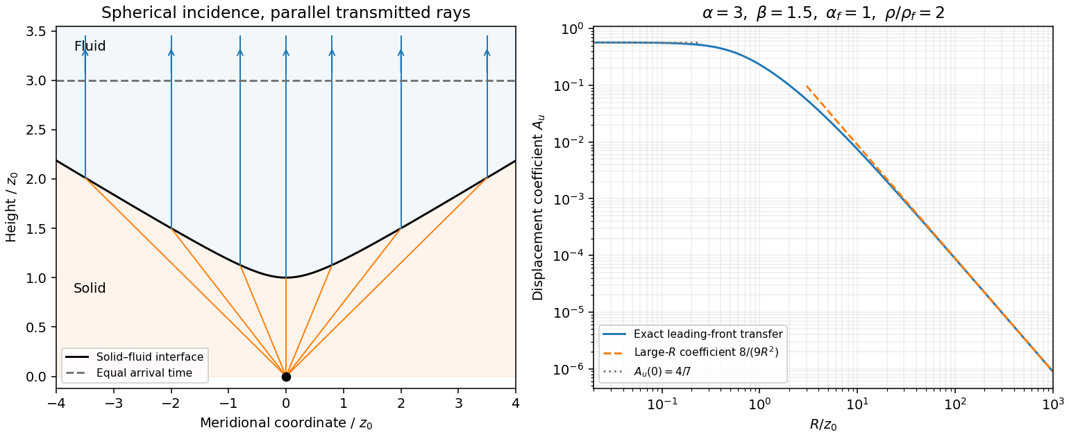
Hyperbolic refraction into vertical rays and the leading transmitted displacement field coefficient compared with its grazing-incidence asymptote
. Details. Past exam of the mathematics course of the University of Cambridge 2004 iii Paper 79 2 iii Solution by Codex 0 Created 2026-10-03 Updated 2026-10-14
Codex 0 Created 2026-10-03 Updated 2026-10-14Use local coordinates with the interface , solid below and fluid above, and choose the P-SV displacement potentials convention , . Let the reflected P and SV potential wave amplitudes be , while the transmitted P wave amplitude is . All four waves have the same tangential slownessThe incident and transmitted retarded times have negative , while elastic waves have positive . At the interface all waveform derivatives therefore have the same argument. displacement field continuity givesWith Lamé parameters and , the shear and normal stresses follow directly from differentiation:The fluid has no shear traction, so the coefficient of in must vanish:The coefficient of in the solid stress is ; in the fluid it is . ThusThese are the three required matching conditions; tangential displacement field need not be continuous at a solid–inviscid-fluid boundary.
Put and . From (2), . In (1), the coefficient of simplifies because . Hence . Substitute this into (3) to obtainTherefore the solid-fluid P-wave transmission coefficient isDivision by was only an elimination device; the final expression extends continuously to . The normal-incidence value is . This is a potential coefficient; longitudinal displacement field transmission additionally multiplies it by . The original PDF's bracket lies in the denominator and contains and . The converted TeX misplaces the bracket, substitutes for , and loses the final cosine.
Past exam of the mathematics course of the University of Cambridge 2004 iii Paper 79 2 ii Solution by Codex 0 Created 2026-10-03 Updated 2026-10-14
Codex 0 Created 2026-10-03 Updated 2026-10-14The angles from part (i) have sinesBy Snell law for elastic and acoustic waves, . Both angles lie in , so . The outgoing fluid ray tilts away from the inward-tilted normal by exactly its tilt from vertical; it therefore travels vertically upwards. This is hyperbolic interface collimation of P-waves.
The source-to-interface distance satisfiesOne can verify this by squaring, using . ConsequentlyAdding the vertical fluid travel time from the interface to height givesThus surfaces of equal arrival time in the fluid are horizontal planes. Their leading wave amplitude may vary with : a planar wavefront does not imply a spatially uniform plane-wave solution at every order.
Past exam of the mathematics course of the University of Cambridge 2004 iii Paper 79 2 i Solution by Codex 0 Created 2026-10-03 Updated 2026-10-14
Codex 0 Created 2026-10-03 Updated 2026-10-14Work in a meridional plane and denote the interface height by , to distinguish it from an observation coordinate. PutThe interface is , so . Its unit normal into the fluid is proportional to . Consequently the angle between this normal and the vertical satisfiesThe outgoing source P wave has ray direction proportional to , tilting outwards by from the vertical, while the normal tilts inwards. Thus . The tangent addition formula givesDirect substitution simplifies its denominator to and its numerator to . HenceThe denominator is positive, so these are the physical incidence angles in ; the transmitted P wave reaches the fluid rather than propagating back into the solid.
Past exam of the mathematics course of the University of Cambridge 2004 iii Paper 77 3 ii Solution by Codex 0 Created 2026-10-03 Updated 2026-10-14
Codex 0 Created 2026-10-03 Updated 2026-10-14The cell conservation equation equates the change of cell number density to minus the divergence of its total flux. The flux is advection by the water, is the mean swimming flux, and is the dispersal flux. The tensor describes effective translational diffusion, whereas in part (i) describes rotational diffusion; they have different dimensions. This conservation law neglects birth, death and sources at the walls.
The equation expresses incompressible flow. In the momentum equation, is the reference suspension density, is material acceleration times density, is the pressure force after subtracting the pure-water hydrostatic pressure, and is the viscous force for constant dynamic viscosity in a Newtonian fluid. Since counts cells per volume, in is excess downward weight per cell; it is not an acceleration. The small cell-fluid density difference permits the Boussinesq approximation: retain that difference in buoyancy while using constant elsewhere. Diluteness permits neglect of cell-cell interactions, changes of viscosity, and active cell stresses. Any separate settling speed is assumed negligible or already incorporated in the specified mean drift. The light strength and swimming speed are uniform.
Consider the intended long-channel bulk approximation. At the sidewalls impose zero normal cell flux and the no-slip boundary condition. The closed ends require zero total fluid flux through each horizontal section, so ; localized turning regions are omitted from the bulk equations. The mean concentration is . The final paragraph below distinguishes these bulk conditions from exact closed-end cell conservation.
For , the vorticity is . Hence , and the leading horizontal mean swimming direction is . With and , steady cell conservation equation says that is constant. Its wall value is zero, so with . The phototactic concentration in a vertical channel is thereforeThis result neglects the correction to horizontal swimming. For positive phototaxis, and cells accumulate towards the illuminated wall .
The steady inertial terms vanish for , since . The horizontal momentum equation gives . The vertical momentum equation then requires a constant excess pressure gradient and gives . Twice integrating producesSet . The two no-slip boundary conditions give and . The zero fluid-flux condition follows by integrating this expression:Consequently the remaining constants areThe resulting velocity can also be written without separate polynomial constants asHere is the zero-flux pressure gradient in a cell-driven channel. It is negative for : pressure decreases upwards, creating the upward pressure force that balances the excess cell weight and drives the return flow. Its magnitude is determined by zero net fluid transport, not by prescribing pressure independently. In the zero-light limit, the continuous result is , and .
For the requested large- sketch, cells occupy a boundary layer of thickness near . Put and . The exact dimensionless profile above isAway from the illuminated-wall layer it tends to . There is broad upward return flow for and downward flow on the illuminated side. The outer maximum is at . Near , the exponential term is approximately and restores the no-slip boundary condition from the negative outer velocity to zero at the wall. The finite- profile shown below retains that layer. The small-vorticity assumption must still be enforced, for example by sufficiently weak excess weight or a sufficiently dilute suspension; alone does not ensure .
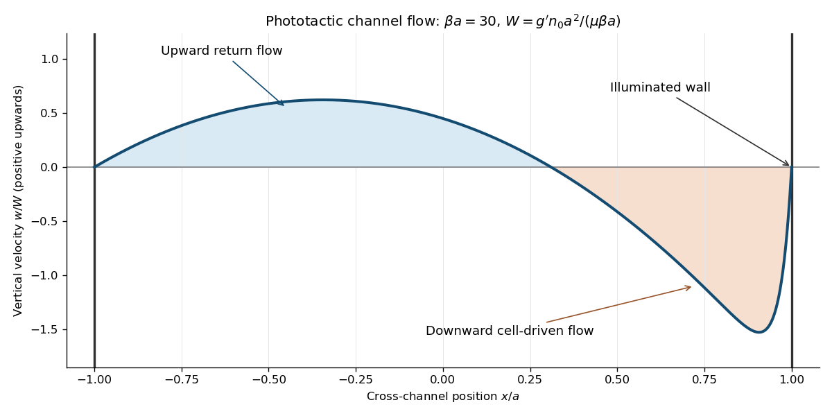
There is a genuine global qualification to the bulk construction. For an exactly steady channel with impermeable ends as well as impermeable sidewalls, the closed-channel cell-flux constraint also requires at every height. In this bulk ansatz the first-order orientation closure givessince integration by parts, and imply . Moreover, multiply by and integrate. The wall values and zero fluid flux givefor a nontrivial profile. Thus zero axial cell flux generally fails unless the extra factor vanishes, or the flow is trivial. A complete steady closed-channel solution generically needs axial concentration variation. The explicit profile solves the stated bulk equations, sidewall conditions, concentration normalization and zero fluid-flux condition; it is not, for arbitrary parameters, an exact globally closed steady cell distribution. Ignoring end regions gives the intended bulk approximation, but does not by itself prove the stronger global existence claim.
Past exam of the mathematics course of the University of Cambridge 2004 iii Paper 77 3 i Solution by Codex 0 Created 2026-10-03 Updated 2026-10-14
Codex 0 Created 2026-10-03 Updated 2026-10-14Neglecting cell rotational inertia, the light and viscous torque sum to zero. Therefore the angular velocity is . A material orientation evolves by . The vector triple-product identity givesThe last term is the projection of onto the tangent plane to the unit sphere. In particular, , as required to preserve the unit orientation. It aligns the swimmer towards the light; the vorticity rotates that orientation.
For rotational diffusion coefficient , the phototactic orientation Fokker-Planck equation balances deterministic orientation drift with diffusion on the sphere. Its density is normalized with respect to solid angle, not . When , there is no azimuthal drift and the zero-current condition is . Thus , and normalization givesThe limiting density at is .
To justify the angular dependence of the first correction, define the operatorsThe steady Fokker-Planck equation is . Its regular expansion therefore givesThe coefficients of are independent of , so each azimuthal Fourier harmonic is preserved. The forcing has only the sine harmonic with azimuthal number one. There can be no extra unforced harmonic in a smooth normalized first correction: writing a homogeneous solution as gives . Multiplication by and integration by parts on the sphere gives , hence is constant. Normalization removes that multiple of . It follows thatNo explicit calculation of is needed. Its dependence is on and the parameter , and its behavior at the poles must make the density smooth.
In the stated spherical coordinates, . Azimuthal integration makes the leading components and the first-order corrections vanish. The surviving coefficients areThus the small-vorticity phototactic orientation response isBoth coefficients depend only on . In particular, is the Langevin function of and is positive for positive light strength; its integral representation above suffices.
Past exam of the mathematics course of the University of Cambridge 2004 iii Paper 77 1 iii Solution by Codex 0 Created 2026-10-03 Updated 2026-10-14
Codex 0 Created 2026-10-03 Updated 2026-10-14A freely swimming body has neither an imposed end couple nor an imposed end transverse force. Its end bending moment is therefore zero, and the transverse force is also zero at both ends. These are the four free-end bending boundary conditions; they do not require the end displacement or slope to vanish.
Put , using the physically consistent sign. Integrating with the two leading-end conditions givesThe two trailing-end conditions consequently requireThese free-end compatibility for a swimming beam conditions are total transverse force and torque balances. They explain why an arbitrary plausible prescribed does not suffice: two integration constants can satisfy only two end conditions unless the forcing already satisfies both compatibility integrals.
The missing freedom is the swimming recoil correction. An observed or prescribed deformation relative to the body must be supplemented by a lateral translation and a small yaw :To identify with the actual centre of mass displacement, first remove the body-mass-weighted mean from . One may also remove its body-mass-weighted first moment about to define the yaw reference uniquely. This changes the decomposition of the observed motion, not the physical displacement.
For , the recoil contribution to the forcing isInsert into the two compatibility integrals, using and as weights. This gives two coupled ordinary differential equations for the two recoil motions. Their principal acceleration matrix isFor a nondegenerate positive mass distribution it is a positive-definite matrix: its quadratic form at is unless . Thus initial translation and yaw determine the recoil through these equations, and the corrected supplies the two compatibility conditions. The four free-end conditions determine the bending moment together with two rigid recoil motions; they do not overdetermine a physically complete swimming motion.
Past exam of the mathematics course of the University of Cambridge 2004 iii Paper 77 1 ii Solution by Codex 0 Created 2026-10-03 Updated 2026-10-14
Codex 0 Created 2026-10-03 Updated 2026-10-14Choose the internal transverse force so that the net internal transverse force on a slice is . Its linear momentum balance is thenThe coordinate labels body slices, so their lateral material acceleration is ; the fluid transport operator must not be substituted for this body acceleration.
Let be the total internal bending moment, including both passive elastic and active muscular contributions. With the compatible moment orientation, the net couple on the slice is . The cross-sectional rotary inertia is smaller than the translational inertia by the square of the transverse-to-longitudinal length ratio, and is neglected in this slender-beam approximation. Slice angular momentum balance therefore gives . Eliminating from the slice linear momentum balance provesThis equation is the balance law for an active bending beam for a swimming fish; a constitutive relation for the passive bending moment or the muscle actuation is not needed to derive it. With the force-on-body convention established above it becomesAs a check, constant and rigid lateral acceleration give the effective inertia . Combining the printed positive force in part (i) with the minus sign in the beam equation would instead give . That is the same sign defect, rather than a negative hydrodynamic added mass. If the positive quantity in part (i) is called as a force on the fluid, the beam equation must contain .
Past exam of the mathematics course of the University of Cambridge 2004 iii Paper 77 1 i Solution by Codex 0 Created 2026-10-03 Updated 2026-10-14
Codex 0 Created 2026-10-03 Updated 2026-10-14The Lighthill elongated-body theory approximation treats each cross-section of a slender swimmer as a locally two-dimensional potential flow problem. The transverse dimension is small compared with the length and the scale over which cross-sections vary. The displacement and slope are small enough to linearize the impermeability condition about a straight body. The Reynolds number is sufficiently large for lateral loading to be dominated by fluid inertia; viscosity, axial friction and higher-order end corrections are neglected at this order. This reactive approximation must be distinguished from the viscous resistive-force theory used for a flagellum.
In coordinates translating with the swimmer, the undisturbed fluid passes in the positive direction at speed . Applying the impermeability condition to the moving centre plane gives the transverse fluid velocityThe local added mass is defined so that the transverse fluid hydrodynamic impulse per unit axial length is . A fixed body-coordinate interval receives an impulse flux at its leading end and loses the corresponding flux at its trailing end. Its rate of change of impulse plus the net outward impulse flux is thereforeThis is the transverse force exerted by the body on the fluid. By Newton's third law, the transverse force exerted by the fluid on the body has the opposite sign:The distinction is essential here: the printed positive expression is labelled as the force on the fish, so that label and expression are inconsistent. For example, take a uniform cross-section and a rigid lateral displacement . The swimmer must accelerate fluid of added mass , which reacts on it with force , not . Thus the positive expression is recovered exactly with the force-on-fluid convention; the physically consistent force on the fish is the negative expression. In the following parts, denotes so that the beam balance uses a genuine external force on the fish.
Past exam of the mathematics course of the University of Cambridge 2004 iii Paper 76 5 b Solution by Codex 0 Created 2026-10-03 Updated 2026-10-14
Codex 0 Created 2026-10-03 Updated 2026-10-14Assume again positive diffusion . Remove the drift with . Differentiating explicitly cancels the first derivative and givesBalance the second derivative with the linear confinement by taking , so the requested exponent is . More precisely, putThe eigenvalue problem reduces to . Its two solutions are Airy functions. The growing is excluded by the condition at infinity: its growth proportional to dominates any linear-in- drift factor. The decaying remains admissible even after multiplication by . The wall imposes , so , giving the Airy global modes of a linearly confined Ginzburg-Landau equation:The least negative zero, , gives the largest temporal growth rate. HenceAt equality the leading global eigenmode is neutral, and below it all these eigenmodes decay. In contrast, freezing the coefficients locally gives absolute hydrodynamic instability wherever . Such a pocket exists iff and extends to . Thus global instability implies a locally absolutely unstable pocket, while the converse fails: a pocket shorter than does not overcome the wall and confinement losses. The additional threshold is order , precisely the loss produced by the Airy function spatial scale.
Pinned article: Introduction to the OurBigBook Project
Welcome to the OurBigBook Project! Our goal is to create the perfect publishing platform for STEM subjects, and get university-level students to write the best free STEM tutorials ever.
Everyone is welcome to create an account and play with the site: ourbigbook.com/go/register. We belive that students themselves can write amazing tutorials, but teachers are welcome too. You can write about anything you want, it doesn't have to be STEM or even educational. Silly test content is very welcome and you won't be penalized in any way. Just keep it legal!
Intro to OurBigBook
. Source. We have two killer features:
- topics: topics group articles by different users with the same title, e.g. here is the topic for the "Fundamental Theorem of Calculus" ourbigbook.com/go/topic/fundamental-theorem-of-calculusArticles of different users are sorted by upvote within each article page. This feature is a bit like:
- a Wikipedia where each user can have their own version of each article
- a Q&A website like Stack Overflow, where multiple people can give their views on a given topic, and the best ones are sorted by upvote. Except you don't need to wait for someone to ask first, and any topic goes, no matter how narrow or broad
This feature makes it possible for readers to find better explanations of any topic created by other writers. And it allows writers to create an explanation in a place that readers might actually find it.
Figure 1. Screenshot of the "Derivative" topic page. View it live at: ourbigbook.com/go/topic/derivativeVideo 2. OurBigBook Web topics demo. Source. - local editing: you can store all your personal knowledge base content locally in a plaintext markup format that can be edited locally and published either:This way you can be sure that even if OurBigBook.com were to go down one day (which we have no plans to do as it is quite cheap to host!), your content will still be perfectly readable as a static site.
- to OurBigBook.com to get awesome multi-user features like topics and likes
- as HTML files to a static website, which you can host yourself for free on many external providers like GitHub Pages, and remain in full control

Figure 2. You can publish local OurBigBook lightweight markup files to either OurBigBook.com or as a static website.
Figure 3. Visual Studio Code extension installation.
Figure 5. . You can also edit articles on the Web editor without installing anything locally. Video 3. Edit locally and publish demo. Source. This shows editing OurBigBook Markup and publishing it using the Visual Studio Code extension. 
- Infinitely deep tables of contents:




All our software is open source and hosted at: github.com/ourbigbook/ourbigbook
Further documentation can be found at: docs.ourbigbook.com
Feel free to reach our to us for any help or suggestions: docs.ourbigbook.com/#contact