Topics (384k) Articles (398k) Users (410) Discussions (242) Comments (383) Files (13k) New article
Past exam of the mathematics course of the University of Cambridge 2010 iii Paper 7 1 Solution by  Codex 0 Created 2026-10-03 Updated 2026-10-14
Let be a closed manifold of even dimension , with a Riemannian metric and a spin structure. Let be its spinor bundle, and let be a Hermitian vector bundle with a unitary connection of vector-bundle curvature . We use Clifford multiplication satisfying , so the Twisted Dirac operatoris self-adjoint and . Here is an oriented local orthonormal basis and its dual. The Atiyah-Singer index theorem in this setting isThe second factor is the Chern character; the first is the A-hat formThe square root has constant term one. All functions of the vector-bundle curvature matrices mean power series truncated above the dimension of . The brackets select the top-degree differential form. The Bianchi identity shows that these forms are closed, and Chern-Weil connection transgression shows that their de Rham cohomology classes do not depend on the chosen connections on a vector bundle.
The global step is supersymmetric quantum mechanics. On the Hilbert space , take the grading operator , the odd supercharge , and the nonnegative Hamiltonian . They obey and . The principal symbol of is invertible away from the zero covector, so elliptic regularity and Rellich-Kondrachov compactness theorem give a smooth discrete orthonormal eigenbasis for , finite-dimensional eigenspaces, and a trace-class operator for . Define its supertrace by .
For every positive eigenvalue of , the map is an isomorphism between its positive and negative grading eigenspaces, with inverse itself. Their contributions to the supertrace cancel. The zero eigenspaces are and . ConsequentlyThis also proves independence of without differentiating an unbounded operator inside a trace. If is the heat kernel, the heat kernel trace formula givesThe remaining task is to compute this local integrand as .
Fix , use geodesic normal coordinates , and trivialize by radial parallel transport. Expanding at gives the Lichnerowicz formula for a twisted Dirac operator:Indeed the terms with identical indices give the rough Laplacian. The other terms are . Decompose this vector-bundle curvature into spin curvature and ; substituting the spin curvature into the Clifford algebra relations and the algebraic Bianchi identity leaves . Thus the calculation retains the curvature of the twisting bundle explicitly.
There is an especially strong cancellation in the spinor supertrace. With , every ordered product of distinct Clifford generators of degree less than has zero supertrace, whileFor an even product of lower degree, conjugate times that product by a missing Clifford generator: it changes sign, so its matrix trace is zero. An odd product exchanges the grading summands and also has zero supertrace. For the full product, , and , giving the displayed constant.
To exploit this, identify the Clifford algebra as a filtered vector space with the exterior algebra by sending an ordered Clifford product to the corresponding wedge product of differential forms. Implement Getzler rescaling: put , , multiply the degree- exterior component of the kernel by , and multiply the whole kernel by . A derivative and a Clifford generator have rescaling degree one; a coordinate has degree minus one. Clifford contractions lower the degree by two relative to the wedge product of differential forms, so the leading product becomes exterior multiplication.
In the radially parallel frame, the linear Taylor term of the connection is determined by its vector-bundle curvature: if is its matrix, then . To check the coefficient, radial gauge means , and integration of along the radial segment gives . Combining this formula with the spin representation, the symmetries of Riemann curvature tensor, and the Lichnerowicz formula for a twisted Dirac operator, the rescaled square has leading modelHere is the skew matrix of tangent-bundle curvature two-forms at ; changing the curvature-matrix sign convention changes the sign inside the covariant derivatives but not the determinant below. The coefficients act in . The scalar-curvature term has degree zero and disappears after multiplication by ; the linear spin-connection term and the Clifford action of have degree two and survive. Higher Taylor terms have smaller degree and disappear.
For clarity, the analytic meaning of this limiting calculation is the following. Construct the local heat kernel expansion to any fixed order and insert the Taylor expansion of the rescaled coefficients into its transport equations. At each exterior degree, the leading equation is the heat equation of ; the remaining terms acquire positive powers of . Equivalently, successive substitutions ingive the same expansion. Polynomial spatial factors are integrable against the local Gaussian kernels, and only finitely many exterior degrees exist. A cutoff outside a fixed normal neighbourhood contributes . Choosing the initial expansion order arbitrarily large bounds its differentiated remainder to any required order. This proves convergence of the rescaled diagonal kernel to the model diagonal kernel, uniformly in on the compact manifold. Its degree- component has no net power of , precisely the component detected by the spinor supertrace.
We can compute the model kernel rather than invoke a local index formula. Set and seek its kernel from the origin in the formThe scalar even exterior coefficients of commute. On this ansatz the rotational first-order term vanishes because is a function of . Expanding the model operator gives , so substitution into the heat equation givesThe Euclidean initial condition , selectsThese expressions have well-defined power series at . This is the curvature version of the Gaussian calculation underlying the Mehler formula for Hermite functions.
At , , multiply the top exterior coefficient by the spinor supertrace constant. Since , and every curvature factor is a two-form, the result isIntegration and the constant supertrace established above prove the boxed Atiyah-Singer index theorem. The mechanism is that odd symmetry pairs the nonzero spectrum globally, while the Clifford filtration makes the surviving local contribution an explicitly solvable curvature oscillator. Odd-dimensional spin Dirac operators have no canonical chiral index of this type; their self-adjoint Fredholm index is zero. For comparison of normalization conventions, Raphaël Ponge's local index calculation writes the same unnormalized curvature model and spinor supertrace constant.
Past exam of the mathematics course of the University of Cambridge 2010 iii Paper 69 4 Solution by Codex 0 Created 2026-10-03 Updated 2026-10-14
Codex 0 Created 2026-10-03 Updated 2026-10-14The case for anthropogenic global warming rests on a physically consistent combination of forcing, energy storage and observed response, rather than on the claim that every unusual event has the same cause. For this examination, the observational comparison is the evidence available around 2010, and the two forecast horizons are approximately 2060 and 2110. Separating the robust mechanisms from uncertain regional details is essential to a coherent attribution of recent climate change.
The greenhouse effect follows from radiative transfer. Sunlight supplies energy, while the Earth loses energy mainly through long-wave radiation. Carbon dioxide, methane and other greenhouse gases absorb and emit in parts of that outgoing spectrum. Increasing their concentrations alters the levels and temperatures from which radiation escapes, initially reducing the net loss of energy for a given surface state. The surface and atmosphere must then warm until outgoing radiation again balances the input. Strong absorption near the centres of some bands does not eliminate the influence of additional gas: absorption in the wings and the changing height of emission still matter. For scale, the approximate carbon dioxide forcing law gives about for doubling. It describes a forcing, not the ultimate temperature response, which additionally involves climate feedbacks and ocean heat uptake.
Measured increases in atmospheric carbon dioxide are consistent with fossil-fuel combustion and changes in land use. The carbon isotope signature and atmospheric oxygen consumption provide independent evidence of the combustion source, while the ocean and land absorb part of the emitted carbon. Methane and other climatically active gases add to the forcing. Aerosols exert partially compensating effects, so net human forcing is smaller than the sum of the warming gases alone. Uncertainty in that compensation affects the quantitative rate of warming without removing the greenhouse mechanism.
A sustained rise in global temperature is accompanied by increased ocean heat content, glacier retreat and sea level rise. This combination is harder to explain as an artefact of a few surface thermometers than a temperature series in isolation: the ocean is a large energy reservoir, and thermal expansion and melting have independent observational consequences. Internal variations of ocean circulation can move heat between regions and alter warming over particular decades, but cannot indefinitely supply a positive global energy accumulation without a change in the energy budget. Solar changes and volcanic eruptions also influence climate, and must be included in attribution; they do not reproduce the full recent warming pattern and sustained heat gain. Volcanic aerosol episodes chiefly produce temporary cooling. Broad troposphere warming together with stratosphere cooling is another useful fingerprint: additional greenhouse gases and ozone changes have a different vertical response from simply increasing solar input. No one fingerprint is unique to one cause, but their joint agreement with greenhouse forcing strengthens the attribution.
Polar observations are especially informative because they connect atmosphere, ocean and ice. In the Arctic, reduced summer sea ice extent, thinning and loss of multi-year sea ice indicate a diminished ice reservoir. Warmer air, earlier melt and delayed freeze-up contribute, while wind and current changes redistribute ice and export thick floes. Pacific heat inflow and changes in Atlantic-origin waters supply oceanic routes to melting. The protection afforded by the cold halocline means that warmer Atlantic water does not automatically heat the ice: the intervening mixing and density stratification must be considered. The 2007 retreat illustrates how long-term thinning, anomalous winds and greater solar absorption can combine. It neither proves that weather variability has ceased nor provides a reason to ignore the longer-term energy imbalance.
Loss of grounded ice has a different global implication. Increased surface melt and runoff on Greenland, and changes in outlet-glacier discharge, transfer water from land to the ocean. In Antarctica, warming of the Peninsula and disintegration of some ice shelves demonstrate strong regional change. Warm ocean water reaching shelf cavities can thin floating shelves from below; loss of ice-shelf buttressing can then speed grounded-ice discharge. The floating shelf's disappearance is not itself equivalent to adding its whole volume to sea level. The important subsequent response is increased loss from grounded ice sheets. Increased snowfall can compensate some losses, so a mass budget must distinguish accumulation, melting and ice flow.
The two polar regions should not be assumed to behave identically. Around 2010, Antarctic sea-ice changes included strong regional contrasts and an overall satellite-era behaviour quite different from Arctic summer retreat. Winds, ozone-related atmospheric changes, freshwater effects and the circulation of the Southern Ocean influence the Antarctic pattern. A large cold continent surrounded by an ocean is physically different from an ocean surrounded by land, and vigorous Southern Ocean heat uptake can delay surface warming. A regional increase in Antarctic sea ice is therefore compatible with global ocean heat gain and losses from some grounded Antarctic ice; it still needs its own dynamical and thermodynamic explanation. Credible attribution accounts for these differences instead of requiring uniform warming everywhere.
Several mechanisms produce polar amplification. The ice-albedo feedback is the most direct: retreating snow and ice expose darker surfaces that absorb more sunlight, causing further warming and melt. Much of the extra energy over newly open Arctic water is stored during summer and released to the atmosphere in autumn and winter, when an ice-covered ocean would be better insulated. Consequently the largest near-surface atmospheric response need not occur in the season of greatest solar input. Sea-ice loss changes both reflection and the timing of ocean heat release.
The atmospheric vertical structure also matters. In the tropics, convective adjustment often produces appreciable warming aloft, which increases radiative cooling. Stable polar boundary layers can concentrate warming near the surface, producing a different lapse-rate feedback and less compensating cooling from upper layers. Furthermore, the idealized Planck feedback scales as : colder emitting regions have a smaller increase of blackbody radiation per kelvin, although a quantitative atmospheric comparison needs full radiative transfer. Water-vapour and cloud changes modify both short-wave and long-wave fluxes, with cloud effects depending on season and surface properties. Changes in poleward heat and moisture transport provide further coupling. Thus polar amplification has several interacting causes; it is not simply the same local ice-albedo process repeated throughout the year.
Polar change affects the rest of the planet. Grounded-ice loss contributes to eustatic sea level change, while ocean warming contributes to thermosteric sea level change; together they increase coastal flooding and erosion risks. Redistribution of ice and freshwater changes density stratification and dense-water formation, potentially altering the Atlantic meridional overturning circulation and other oceanic heat and carbon transports. A weakening is physically plausible under warming and freshening, but an immediate complete shutdown is not a necessary prediction. Permafrost carbon feedback can release additional carbon dioxide and methane, increasing warming outside the Arctic. Habitat loss, changing primary production and altered food webs affect marine ecosystems and people, while a longer open-water season changes navigation, coastal exposure and resource access. These impacts are not exhausted by a single global-mean temperature number.
Forecasts require an emissions scenario as well as physical understanding. On the roughly fifty-year horizon, continued emissions imply further ocean and atmospheric warming, a longer Arctic melt season, less late-summer ice and a greater fraction of young seasonal ice. Mountain glaciers generally continue to lose mass, and sea level continues rising through thermal expansion and land-ice loss. Variability can interrupt a regional trend for several years, and the exact first nearly ice-free Arctic summer cannot be fixed from the 2007 minimum. Ocean heat storage and slow ice-sheet adjustment also mean that some further change is committed even if emissions are reduced.
By approximately 2110, sustained high emissions would imply a substantially warmer world, potentially several degrees above early twenty-first-century global temperatures, with stronger Arctic warming and likely recurrent nearly ice-free late summers. This is a seasonal prediction, not a claim that the entire Arctic Ocean must be ice-free in winter. Losses of grounded ice and thermal expansion would produce larger cumulative sea level rise, plausibly measured in several decimetres and potentially more if ice dynamics accelerate. The largest uncertainty is not whether adding heat expands water, but the future emissions trajectory and the response of major ice sheets. Complete loss of Greenland on this century-long horizon is not required by that prediction. With strong mitigation, substantially smaller late-century warming and ice loss are possible, although sea level can continue to rise beyond stabilization of surface temperature.
Anthropogenic forcing explains the broad warming signal; feedbacks amplify polar change, while emissions and ice dynamics govern future outcomes. This distinction permits both a firm physical conclusion and honest uncertainty about dates, regional details and the magnitude of rapid ice-sheet change.
Past exam of the mathematics course of the University of Cambridge 2010 iii Paper 69 2 Solution by Codex 0 Created 2026-10-03 Updated 2026-10-14
Codex 0 Created 2026-10-03 Updated 2026-10-14A steric sea level change is caused by a change of water volume at fixed ocean mass. Warming usually lowers seawater mass density, producing thermosteric sea level change; freshening also lowers density and produces a halosteric contribution. Both depend on the temperature, pressure and salinity dependence of the equation of state. Regional freshening or warming can therefore change local sea level even when the global ocean mass has not increased.
An eustatic sea level change concerns the ocean water amount or basin capacity. On the coming-century timescale, the principal positive mass contributions are melting mountain glaciers and ice caps, and loss of grounded ice from Greenland and Antarctica, including iceberg discharge. Terrestrial water storage also matters: groundwater depletion transfers water to the ocean, whereas reservoir filling retains it on land. Snowfall accumulation can partly compensate ice loss. Basin changes associated with geology matter over longer periods, and vertical land motion changes locally measured relative sea level. Melting floating sea ice has already largely displaced its eventual meltwater volume; its direct contribution is small compared with transfer of grounded ice into the ocean. Small density and salinity corrections do not alter that distinction.
For scale, a contemporary budget available in 2010 gave the following approximate contributions for 1993–2003, in :These are period-specific estimates with appreciable uncertainties, particularly for Antarctica, rather than exact closure of the budget. For comparison, over 1961–2003 the observed rate was about and the estimated thermal expansion contribution about . The shorter interval need not define a permanent acceleration by itself, but the magnitudes show that thermal expansion and land-ice loss are both essential.
With continued warming, increasing ocean heat content sustains thermosteric sea level change, including after surface warming slows because the deep ocean equilibrates gradually. Increased ice ablation generally increases glacier runoff, although small glaciers eventually lose much of their available ice. Surface melt and changes in outlet-glacier flow can increase the ice-sheet contribution; ocean-driven loss of ice shelves can accelerate discharge of grounded ice. Greater snowfall provides some compensation but cannot be assumed to cancel these losses. Thus, under continued substantial greenhouse gas emissions, the global rate is likely to rise above its historical few millimetres per year, with an increasing contribution from the great ice sheets. The precise century-scale increase depends on emissions, ocean heat uptake and ice sheet dynamics; a single fixed rate extrapolated from one decade is inadequate.
For the idealized mixed-layer calculation, the stated density response givesAt fixed column mass, , so to first orderThis is only the thermosteric sea level change from the prescribed layer and warming. The much larger total observed rise since the nineteenth century does not, by itself, prove deeper warming: part of that rise is eustatic sea level change. After independently allowing for the mass contribution, a larger remaining steric signal would require warming below , a different temperature distribution, or corrections to the simplified equation of state. Direct temperature profiles do independently establish subsurface ocean warming. It reaches depth through winter mixing and open-ocean convection, especially in the North Atlantic and parts of the Southern Ocean; through subduction of surface waters into the interior; and through advection and turbulent mixing. Formation and spreading of intermediate and deep waters transmit surface properties far beyond the immediate region of heat uptake. Warm surface water need not simply sink locally: cooling, freshwater effects and density stratification govern the actual pathways.
Using , the ocean area is . A liquid runoff volume givesThis is the contribution from that input, before allowing for other exchanges in the global ocean freshwater budget.
For the sea-ice dilution estimate, the ocean volume is . Let its initial mean salinity be ; the question does not specify it, so use psu for a numerical estimate. Interpret the as liquid freshwater-equivalent melt, with . Salt mass remains fixed while liquid water mass increases, givingConsequentlyApproximating the densities as equal gives psu per year. If the quoted volume instead denotes literal solid-ice volume, use for the added mass; with the result is psu per year. Either convention gives the same order of magnitude. Floating-ice melt can change mean ocean salinity even though its direct sea-level effect is small: displaced volume and dissolved salt concentration are different budgets.
An observed net freshening is a statement about the sum of all freshwater exchanges, not a separate measurement of every positive contribution. Let be liquid ocean mass, net freshwater runoff from land, net global sea-ice melt minus formation, and net precipitation minus evaporation, all expressed as masses per unit time. The global ocean freshwater budget and salt conservation giveThe runoff term must include non-ice river input as well, or those other exchanges must already have been netted out. If the measured freshening equals that predicted from alone, positive runoff is still possible providedor an equivalent compensating term exists in the complete budget. For instance, excess evaporation can remove water at the same rate at which land-ice runoff supplies it; compensating net ice formation elsewhere must also be included if was initially only the Arctic contribution. Gross seasonal melt cannot be compared with an annual global trend without subtracting refreezing. Such compensation also means that the runoff-only sea-level increment need not equal the total retained increment. If runoff is additional, sea-ice melt is already net and global, and every other freshwater term is zero, the two contributions must add: under those stronger assumptions the alleged equality would be inconsistent. The apparent paradox is resolved by closing the complete freshwater and salt budgets.
Past exam of the mathematics course of the University of Cambridge 2010 iii Paper 69 1 Solution by Codex 0 Created 2026-10-03 Updated 2026-10-14
Codex 0 Created 2026-10-03 Updated 2026-10-14The solar constant measures the incident power per area normal to the sunlight. A spherical Earth of radius intercepts sunlight over the disc , but radiates over its surface . For uniform surface albedo in the global energy-budget approximation, absorbed power is . Treat the surface as a blackbody, assume efficient heat redistribution and neglect internal heating. The Stefan–Boltzmann law and the planetary surface energy balance then giveFor a nonuniform surface the same power balance instead defines an effective planetary equilibrium temperature, ; its fourth root is not generally the arithmetic mean of the local temperatures. Also, area-averaging the surface albedo is an approximation to the properly insolation-weighted averaging. These are the simplifications implicit in the naked-planet calculation.
Take , so . The changed area is , givingThe initial planetary equilibrium temperature is . ThusThe differential estimate gives the same result. This is the global equilibrium response of the specified model, not the immediate local Arctic warming or the full atmospheric response.
The exceptional 2007 Arctic sea ice decline is best understood as a weather event acting on an already vulnerable ice cover, with several reinforcing pathways. Warmer air increases downward long-wave heating, lengthens the melt season and delays autumn freezing. Changes in snowfall and the development of melt ponds also change the surface energy balance. Air temperature alone, however, does not identify the source of the observed bottom melt: heat must reach the underside through the ocean.
Warmer Atlantic-origin water supplies a larger subsurface ocean heat content after entering through Fram Strait and the Barents Sea. Its influence on sea ice depends on vertical exchange, because a cold, relatively fresh halocline normally separates it from the ice. Erosion of that halocline, through altered freshwater distributions, wind-driven mixing or changes in circulation, weakens stable density stratification and can increase upward ocean heat flux. A warmer Atlantic layer without this exchange need not produce immediate extra bottom melt. Conversely, warmer Pacific inflow through Bering Strait introduces heat into the shallower western Arctic; advection through the Chukchi Sea provides another route to ice retreat and ocean heat storage.
The Arctic Oscillation changes winds, ice motion and export. Positive phases during earlier years helped remove old, thick ice through Fram Strait and left a younger, thinner pack. Summer 2007 also had a pronounced pressure contrast between the Beaufort region and the Eurasian Arctic, associated with the Arctic dipole anomaly. Its winds promoted ice displacement and warm-air transport. The summer circulation should not be described merely as a particular Arctic Oscillation index: the spatial pattern and the preconditioning from earlier years both matter.
Long-term thinning reduces the latent heat of fusion needed to remove the remaining ice. Replacement of multi-year sea ice by first-year sea ice therefore makes a given summer heat input more effective, while mobile thin ice is more readily redistributed or exported. These dynamical changes can expose open water early enough for substantial solar absorption. Water and melt ponds have lower surface albedo than snow-covered ice, so absorbed short-wave energy rises, increasing upper-ocean heat storage and bottom melt. This ice-ocean albedo feedback also delays refreezing. In the Beaufort Sea in 2007, enhanced solar heating of the newly exposed upper ocean was an especially important explanation of extreme bottom melt. Thus thinning and wind-driven opening can initiate retreat, while solar heating amplifies it; changes in Atlantic or Pacific heat supply can further reinforce the process where circulation permits.
A further positive climate feedback involves terrestrial carbon. Loss of the insulating ice cover permits greater autumn and winter transfer of stored ocean heat to the atmosphere. The resulting regional warming can increase thaw of coastal and inland permafrost. Microbial decomposition of previously frozen organic material then releases carbon dioxide, and oxygen-poor wet environments also release methane. These greenhouse gases strengthen the greenhouse effect, increasing global warming and further thaw. The permafrost carbon feedback provides the causal chain from summer ice retreat to an additional global influence. An Arctic methane feedback involving subsea sources is also possible, but the amount actually reaching the atmosphere depends on oxidation and transport; an abrupt, wholesale release is not a necessary consequence of summer ice loss.
For the bottom-melt estimate, use and the given . Assume the ice at the melting interface is already at its local freezing temperature; there is then no separate sensible-heating term. Per square metre the latent heat requirement isJuly through September has days, so the mean ocean heat flux to the ice isUsing instead gives about , within the intended accuracy. Around the date of this examination, the estimated net anthropogenic radiative forcing since preindustrial times was about ; doubling carbon dioxide gives about . The calculated bottom flux is tens of times larger. There is no energy-budget contradiction: it is a local, summer ocean-to-ice heat transfer, supplied by absorbed sunshine, stored heat and transport, whereas radiative forcing is a global perturbation to the radiation budget. Redistribution and local absorption can produce much larger regional fluxes than the global forcing.
For an already ice-free water column, take and liquid-water specific heat capacity . Assuming all the same energy remains in that uniformly mixed column,If the water initially lies near the seawater freezing point, about , its final temperature is approximately . An absolute final temperature requires that additional initial condition; the energy calculation itself determines only the temperature increase. The given ice specific heat capacity is not the appropriate value for heating liquid seawater.
Past exam of the mathematics course of the University of Cambridge 2010 iii Paper 68 2 Solution by Codex 0 Created 2026-10-03 Updated 2026-10-14
Codex 0 Created 2026-10-03 Updated 2026-10-14Let and suppose stays positive and sufficiently smooth in the region considered. Write in . The leading and first transport equations of the WKB approximation areWith , they give and . Thus the leading WKB approximation for a slowly varying oscillator isThe amplitude is fixed by the transport equation, not just by replacing the constant wave number in a sinusoid. The local validity condition is that variation of over a wavelength is small, for example .
If , the same calculation gives the evanescent formAt a classical turning point where vanishes, these amplitudes diverge and the separated WKB descriptions cease to be uniform. For a simple zero, an Airy turning-point connection formula replaces them in an interval in ; it connects oscillation to exponential behavior with the usual quarter-phase shift. A higher-order zero needs a different local canonical problem, so the Airy statement assumes a simple turning point.
For a smooth positive weight on the closed interval, let . The local wave number in the Sturm-Liouville problem is , and the condition at zero selects a sine. Imposing the condition at gives the WKB quantization conditionFor weighted normalization , rapidly oscillating averaging gives . There is no turning-point phase correction here because stays positive at both endpoints with Dirichlet boundary conditions.
In the specified example , so and . To solve exactly, set and . Direct differentiation reduces the Euler-Cauchy equation to on , with zero endpoint values. Hence the inverse-square weighted Dirichlet spectrum isValues give no nonzero solution satisfying both endpoint conditions. The WKB eigenfunction shape after leading quantization is actually identical to this exact shape; the leading eigenvalue omits .
Using the exact eigenvalue as the reference, its relative error isThus is sufficient and necessary among positive integers. Referencing the approximate value instead gives , and the same integer answer.
Past exam of the mathematics course of the University of Cambridge 2010 iii Paper 67 3 Solution by Codex 0 Created 2026-10-03 Updated 2026-10-14
Codex 0 Created 2026-10-03 Updated 2026-10-14First find the positive spatially homogeneous equilibrium. Setting the reactions to zero gives and , and hence the unique positive equilibrium isThe zero pair is not an admissible positive state and is singular in the term. For homogeneous deviations, the reaction Jacobian matrix at this equilibrium isThus , , and its eigenvalues areFor , both real parts are negative: a real pair has positive product and negative sum, while a complex pair has real part . The reaction equilibrium is therefore asymptotically stable, with no growing oscillatory mode. This does not exclude damped oscillations. Indeed, for the eigenvalues are complex; for example, gives , a stable focus with oscillatory transients. Thus a literal exclusion of every oscillatory solution is false; the intended exclusion of sustained or growing oscillations is the meaningful statement.
One can strengthen this to exclude nonlinear periodic oscillations in the positive quadrant without relying only on the local linear stability analysis. For the reactions , , use the Dulac function . ThenWere there a periodic orbit wholly in the positive quadrant, the flux of through it would vanish, since this vector is tangent to the orbit; Green's theorem would equate that flux to a strictly negative interior integral. This contradiction proves there is no sustained positive periodic oscillation when , the positive-quadrant Dulac multiplier for quadratic activation argument. It leaves the damped transients entirely consistent with the conclusion.
Now introduce a perturbation in the quadratic activator-inhibitor model. The Fourier mode of squared wavenumber evolves underIts matrix trace and determinant areA Turing instability must start with reaction stability, requiring . Then for every , so a mode is unstable exactly when : its two real eigenvalues have opposite signs. This also proves the diffusion-driven onset is stationary rather than oscillatory.
The upward-opening quadratic has its minimum at . To have a negative value at a physically allowed positive squared wavenumber, one needsWriting , the second inequality is , with roots . The first inequality discards the lower branch, givingThese are the Turing threshold of the quadratic activator-inhibitor model conditions. Equivalently, in the plane the instability region lies strictly above and strictly to the left of , with . The boundary diverges as and approaches as .
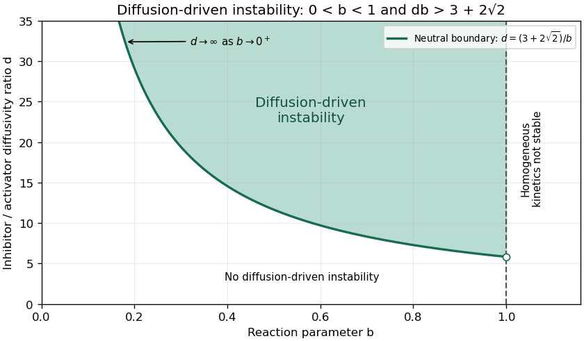
Diffusion-driven instability above the quadratic-model threshold in the reaction-stable parameter strip
. Details. At equality, the determinant has a double root and one growth rate is zero, while the other remains negative. Substituting into its minimum location givesBeyond onset, the unstable band isThe stated parameter region assumes continuously available wavenumbers, as on an infinite domain. With specified finite-domain boundary conditions, an allowed nonzero spatial eigenmode must additionally lie in this band; homogeneous stability alone does not ensure that a finite box admits the critical wavelength.
Pinned article: Introduction to the OurBigBook Project
Welcome to the OurBigBook Project! Our goal is to create the perfect publishing platform for STEM subjects, and get university-level students to write the best free STEM tutorials ever.
Everyone is welcome to create an account and play with the site: ourbigbook.com/go/register. We belive that students themselves can write amazing tutorials, but teachers are welcome too. You can write about anything you want, it doesn't have to be STEM or even educational. Silly test content is very welcome and you won't be penalized in any way. Just keep it legal!
Intro to OurBigBook
. Source. We have two killer features:
- topics: topics group articles by different users with the same title, e.g. here is the topic for the "Fundamental Theorem of Calculus" ourbigbook.com/go/topic/fundamental-theorem-of-calculusArticles of different users are sorted by upvote within each article page. This feature is a bit like:
- a Wikipedia where each user can have their own version of each article
- a Q&A website like Stack Overflow, where multiple people can give their views on a given topic, and the best ones are sorted by upvote. Except you don't need to wait for someone to ask first, and any topic goes, no matter how narrow or broad
This feature makes it possible for readers to find better explanations of any topic created by other writers. And it allows writers to create an explanation in a place that readers might actually find it.
Figure 1. Screenshot of the "Derivative" topic page. View it live at: ourbigbook.com/go/topic/derivativeVideo 2. OurBigBook Web topics demo. Source. - local editing: you can store all your personal knowledge base content locally in a plaintext markup format that can be edited locally and published either:This way you can be sure that even if OurBigBook.com were to go down one day (which we have no plans to do as it is quite cheap to host!), your content will still be perfectly readable as a static site.
- to OurBigBook.com to get awesome multi-user features like topics and likes
- as HTML files to a static website, which you can host yourself for free on many external providers like GitHub Pages, and remain in full control

Figure 2. You can publish local OurBigBook lightweight markup files to either OurBigBook.com or as a static website.
Figure 3. Visual Studio Code extension installation.
Figure 5. . You can also edit articles on the Web editor without installing anything locally. Video 3. Edit locally and publish demo. Source. This shows editing OurBigBook Markup and publishing it using the Visual Studio Code extension. 
- Infinitely deep tables of contents:



All our software is open source and hosted at: github.com/ourbigbook/ourbigbook
Further documentation can be found at: docs.ourbigbook.com
Feel free to reach our to us for any help or suggestions: docs.ourbigbook.com/#contact