Topics (384k) Articles (398k) Users (410) Discussions (242) Comments (383) Files (13k) New article
Past exam of the mathematics course of the University of Cambridge 2009 iii Paper 72 7 Solution by  Codex 0 Created 2026-10-03 Updated 2026-10-14
A fixed-step linear multistep method for uses several previous solution and derivative values:The coefficients are fixed independently of the step size. It is explicit when and implicit otherwise. Its characteristic polynomials of a linear multistep method are and . The contraction mapping theorem gives a uniquely solvable implicit step under a Lipschitz continuity bound whenever , by contraction of the new-value equation on the appropriate solution region. A suitable starting procedure must supply the first values; the method alone does not determine them.
Order is defined by inserting a smooth exact solution into the recurrence. If the residual is and its first nonzero coefficient occurs at that degree, the method has order ; dividing the residual by gives an local truncation error. Taylor expansion gives the exact order conditions for a linear multistep methodwith the right side interpreted as zero at , and failure at for exact order. Equivalently,The basic consistency of a numerical method conditions are , ; for the ordinary nondegenerate consistent formulation this common value is nonzero. Exactness on constants and linear functions does not control propagation of numerical perturbations.
That propagation is the role of zero-stability. On the homogeneous recurrence is . Its modes are , with powers of determined by root multiplicities. The theorem on the root condition for a multistep method states that zero-stability is equivalent to every root of having modulus at most one, with every unit-modulus root simple. Interior repeated roots are permitted, since geometric decay dominates their polynomial factors. An exterior root amplifies perturbations geometrically; a repeated unit root amplifies them polynomially and violates a step-independent perturbation bound.
The Dahlquist equivalence theorem states that a fixed-step consistent linear multistep method is convergent exactly when it is zero-stable. This concerns ordinary differential equations with a uniformly Lipschitz continuous right-hand side on the solution region over a fixed finite interval, convergent starting values, and the well-defined nearby branch of each small-step implicit solve. For order convergence of a numerical method, the solution must have the required smoothness and the starting errors must be .
The mechanism can be sketched explicitly. The root condition for a multistep method bounds the recurrence's discrete Green function. For an order- exact-solution defect , the Lipschitz continuity error equation then gives an estimate of the formThe current-step term can be absorbed for small . The discrete Gronwall inequality says that a bound implies . There are defects on a fixed interval, so their sum is and this yields the claimed global order. Conversely, testing with vanishing starting perturbations in exterior-root or repeated-unit-root modes proves that convergence of a numerical method fails without the root condition for a multistep method.
For example, the two-step Adams-Bashforth method hasIt is explicit, order two and zero-stable, hence convergent with order-two starting values. By contrast, a recurrence with has solutions on the zero differential equation. Starting differences tend to zero yet become unbounded at a fixed positive time, since is of order . A small local defect or formal high order cannot rescue this mode. Canceling a common factor may remove it only by changing the allowed starting relations, as the parameter endpoint in Question 2 illustrates.
Absolute stability addresses a different limit: apply the method to the Dahlquist test equation and put . The amplification roots satisfyAll roots must satisfy the disk condition, with unit roots simple; one cannot inspect only the root that tends to one as . The degree and solvability of the recurrence must also be preserved. The resulting set of is the domain of absolute stability. A-stability means that it includes the whole closed left half-plane, so the numerical solutions of every Dahlquist test equation with are stable for every positive step size. It is a linear test-equation property, not a proof of arbitrary nonlinear contractivity or high accuracy at large steps.
Forward Euler method has order one and factor , so its stability region is the disk . Backward Euler method has factor and is A-stable. The trapezoidal rule is order two with factor ; its modulus is at most one throughout the left half-plane. These one-step methods are included as the simplest multistep examples. For the two-step Adams-Bashforth method, the negative-real stability interval is : its polynomial is , and the root reaches at . It therefore imposes a step restriction when applied to strongly decaying modes.
The genuinely two-step BDF2 method isIt has order two, roots at zero step and is A-stable. For its normalized polynomials , , the unit-circle boundary locus hasThe leading coefficient has no zero in the left half-plane, and the roots at a small negative are both inside the disk. Root continuity then proves open-half-plane stability; on the imaginary boundary the only possible unit root is the simple root one at . This gives a direct proof of the stated A-stability rather than relying on a boundary plot.
Two sharp order barriers explain the tradeoff. The first Dahlquist barrier states that a consistent zero-stable real linear -step method using only first derivatives has order at most for odd and for even ; an explicit method has order at most . The Second Dahlquist barrier states that an irreducible A-stable real linear multistep method has order at most two. These statements concern fixed constant coefficients and the ordinary first-derivative multistep class, not multiderivative methods or arbitrary variable-step formulations. Thus higher order alone is not a route to unconditional stiff stability. Question 2 provides a concrete illustration: its third-order member is zero-stable but not A-stable.
No nontrivial consistent explicit multistep method is A-stable. Its amplification polynomial of a multistep method has a fixed highest coefficient, while at least one lower coefficient grows without bound as real . Were all roots uniformly in the unit disk, their elementary symmetric polynomials would keep all the monic coefficients bounded, a contradiction. This is the coefficient argument behind explicit multistep methods cannot be A-stable.
In practice, selecting a method therefore involves accuracy, startup, the presence of a stiff differential equation, implicit-solve cost and step-size control. Zero-stability handles propagation as the step tends to zero; consistency of a numerical method supplies a vanishing defect; A-stability handles the numerical solutions of all decaying Dahlquist test equations at finite steps. None substitutes for the others, and variable steps or PDE discretizations require additional uniform stability arguments appropriate to their setting.
Past exam of the mathematics course of the University of Cambridge 2009 iii Paper 72 6 Solution by Codex 0 Created 2026-10-03 Updated 2026-10-14
Codex 0 Created 2026-10-03 Updated 2026-10-14The eigenvalue stability analysis of a finite difference method reduces a linear evolution discretization to its modal behavior, but it must retain the norm and the dependence on the mesh. For a homogeneous system obtained by the method of lines, , the solution is . A one-step time discretization gives ; for a Runge-Kutta method, where its stage matrices are invertible, . With a multistep method one instead uses an amplification matrix on the augmented vector of several time levels.
The relevant finite-time stability estimate iswith independent of the refining spatial mesh and allowed time steps. Similarly, semidiscrete stability requires for . The norm should represent the continuum problem, such as the discrete L2 norm in one dimension. A fixed finite matrix having decaying solutions as is not by itself a mesh-uniform result for the partial differential equation.
If , thenThus eigenvalues of modulus at most one give a uniform bound when the diagonalizing bases have uniformly bounded condition numbers. For a normal matrix in the chosen inner product, the spectral theorem for normal operators supplies an orthonormal basis, so the condition number is one and the norm of is exactly . For a self-adjoint or skew-adjoint spatial matrix, applying a scalar stability function preserves this favorable modal structure. This is the setting where eigenvalue calculations provide especially clean, reliable step restrictions.
A precise fixed-matrix statement is also useful: a matrix is power bounded for all nonnegative integers if and only if all its eigenvalues lie in the closed unit disk and every Jordan block at a unit-modulus eigenvalue has size one. Indeed, powers of an interior Jordan block contain a polynomial in times a decaying geometric factor and are bounded; a larger block on the unit circle produces unbounded polynomial growth. For a family of matrices, the resulting bounds must still be uniform. Moreover, finite-time stability versus power boundedness distinguishes this all-time condition from the physical-time estimate above. For example , , has , bounded for despite a nontrivial Jordan block at one. Even the scalar update is stable on fixed intervals, since , although it represents a growing equation rather than a contraction.
For a constant-coefficient periodic difference operator, Fourier modes diagonalize the spatial matrix. The discrete Fourier transform is a unitary operator, so Parseval's identity identifies its modal maximum with the operator norm. The eigenvalue stability analysis of a finite difference method then becomes von Neumann stability analysis. For the Dirichlet discrete Laplacian, a discrete sine transform plays the same role. These facts explain its advantages: a large matrix calculation becomes a scalar symbol or a known spectral interval, and the extremal eigenvalue directly determines a safe time step.
As a first example, centered space discretization of the heat equation has eigenvaluesForward Euler method gives with . Requiring all factors in yields for all periodic meshes. In two dimensions the corresponding uniform bound is . Because these are normal matrices, these scalar bounds prove contraction rather than merely suggest it.
Backward Euler method has , so the centered discretization of the heat equation is contractive for every . The Crank-Nicolson method has and is likewise contractive for these negative real modes. However, its factor tends to for very stiff modes, leaving high-frequency oscillations weakly damped; Backward Euler method tends to zero. The eigenvalues therefore expose the presence of stiff differential equations and damping as well as binary stability. Unconditional stability does not remove accuracy requirements.
For an advection equation example, the upwind finite difference scheme for , , has factor , with . Sinceit is a contraction in the periodic discrete L2 norm exactly for . In contrast, Forward Euler method with centered advection has factor . Its modulus exceeds one at nonzero active frequencies, and repeated amplification makes it unstable under fixed nonzero Courant refinement. A much smaller scaling can bound its finite-time growth, demonstrating again that exact contraction and the most general stability estimate are different claims.
The major limitation is the possible presence of a nonnormal matrix. For example,Both eigenvalues are negative, yet at the second unit vector is amplified by at least . This proves that negative spectra do not imply uniform semidiscrete stability. Ill-conditioned eigenvectors, Jordan normal form and transient amplification can invalidate a spectral-only argument. Direct energy estimates or estimates for the resolvent can supply the missing norm control.
Boundary conditions are another limitation. A periodic symbol proves a periodic or whole-line result, not an arbitrary initial-boundary-value problem. Boundary closure of a difference scheme can introduce growing modes or mesh-dependent amplification. A spatial operator with variable coefficients can still be studied through its assembled matrix, but then whether it is a normal matrix, its condition number and the physical inner product must be checked rather than borrowed from a Fourier stability analysis. For the finite element method the natural mass matrix inner product often turns a generalized eigenvalue problem into a self-adjoint one.
For time-dependent or split updates, separate spectra are insufficient to control products. For instance, and each have only zero eigenvalues, while has eigenvalue . For , alternating the two is unstable. A common contractive norm would control the products, but their individual eigenvalues do not.
Finally, stability and consistency of a numerical method have different roles. The Lax equivalence theorem states that, for a well-posed linear initial-value problem and a consistent finite difference method on compatible grid spaces, stability on every fixed time interval is equivalent to convergence of a numerical method as the admissible meshes refine. Bounded grid representation and the correct initial and boundary setup are part of that framework. An eigenvalue estimate can establish its stability hypothesis in the favorable settings described above; it neither proves consistency of a numerical method nor bypasses its uniformity requirements. The method is therefore a powerful modal tool, provided its spectral calculation is connected to a genuine norm estimate.
Past exam of the mathematics course of the University of Cambridge 2009 iii Paper 71 3 Solution by Codex 0 Created 2026-10-03 Updated 2026-10-14
Codex 0 Created 2026-10-03 Updated 2026-10-14Take the negative-exponential Half-range Fourier transform and setThe advection-diffusion equation has the local relation with flux . Integration over the half-line gives the half-line drift global relationFor the upper decay domainwrite . It is the region above , in particular above . Its boundary is oriented from upper-left infinity through to upper-right infinity, with the domain on the left. Fourier inversion and deformation of the boundary terms giveUse the dispersion symmetry elimination of a boundary trace . It preserves and maps into the lower half-plane. Because , the global relation at impliesThe last term contributes an holomorphic upper-domain integral multiplied by , so it vanishes upon closing the contour for . The solution representation with only known data is consequentlyFor the boundary value , direct integration givesThis quotient is an entire function of when its apparent singularities at are filled by their limits. Those points are not genuine forcing poles of the finite-time transform.
To obtain an exponentially decaying spectral integrand, choose and the exponential-decay contour for half-line drift diffusionDeform to . No pole is crossed: the initial-data denominator in that boundary integral has its only pole at , which lies below since . The apparent singularities of the forcing transform are removable. In the swept outer sectors, has the appropriate bounded growth for the deformation. The contour formula becomesEvaluate the second quotient as a removable expression at , rather than splitting it into artificial residue terms. On either ray,Since , the transient factors have Gaussian decay as . The nontransient forcing term is and thus also decays exponentially for every . The real-axis integral has the Gaussian factor . These estimates provide the requested improvement over integration along .
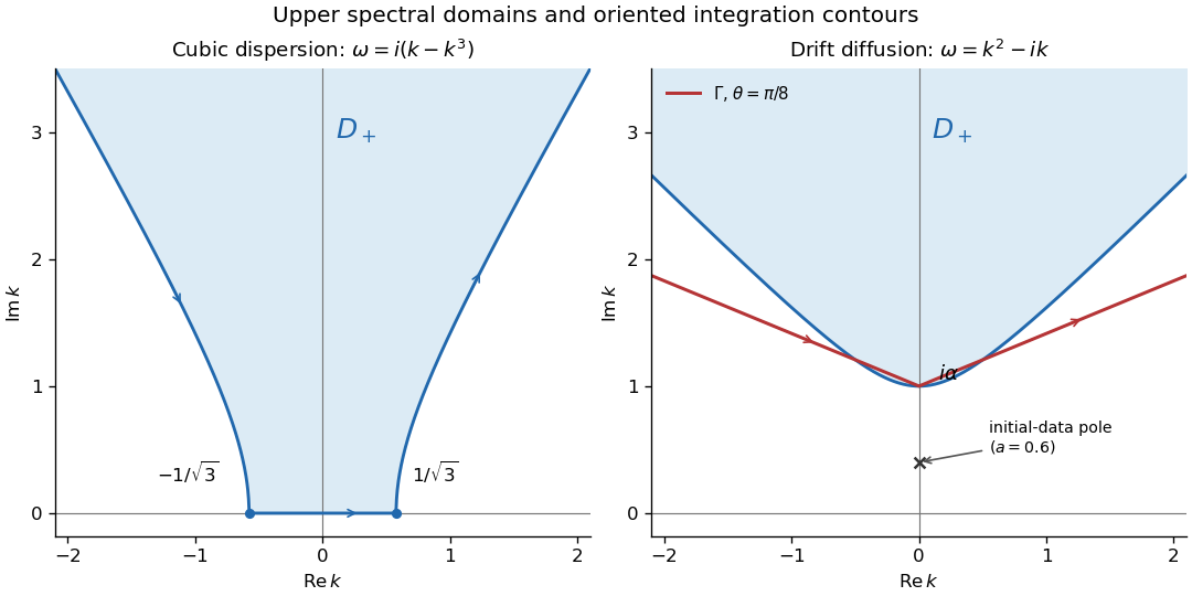
Upper cubic-dispersion contour and exponentially decaying drift-diffusion contour, with their orientations
. Details. The first panel shows the cubic domain from Question 1. The second uses and ; its marked initial-data pole corresponds to and lies below both boundary contours.
An independent real-kernel form also makes the initial and boundary traces explicit. Apply the Dirichlet gauge transform for constant drift, , and then multiply by to obtain the heat equation. The odd-reflected heat kernel for initial data and its Dirichlet boundary-forcing heat-kernel formula yieldThe first kernel tends to the initial delta kernel on as and vanishes at . For the second kernel, the substitution gives the unit-mass approximate boundary delta as , so its trace is ; it vanishes initially for fixed . Differentiating the kernels for verifies the advection-diffusion equation. The integrals converge for every positive , even when the exponentially weighted initial datum grows, because the spatial Gaussian controls that growth. Thus this gives the same decaying solution without introducing an additional restriction on .
For a general decaying initial datum, an unweighted Fourier sine transform does not directly diagonalize the drift operator. DefineTwo integrations by parts for and one for giveThe cosine transform remains unknown, so this is not a closed sine-transform evolution. In contrast, the weighted sine transform for half-line drift diffusion of is closed:When the weighted initial transform exists, Fourier sine inversion gives . This method requires suitable decay of , not merely decay of . For the exponential datum it is an ordinary integrable sine transform only when . At one would need a generalized or regularized transform instead; the contour and real-kernel formulas above already work without that restriction. Therefore the ordinary sine transform of is not a closed solution method; a weighted sine transform works under the stated extra weighted-decay condition.
Past exam of the mathematics course of the University of Cambridge 2009 iii Paper 71 2 Solution by Codex 0 Created 2026-10-03 Updated 2026-10-14
Codex 0 Created 2026-10-03 Updated 2026-10-14Use the Wirtinger derivatives and . The Laplace equation gives , so writewhere is holomorphic in the first quadrant and is holomorphic in the fourth quadrant. They are independent functions: the data may be complex, so a complex-conjugation relation between them cannot be assumed.
Let , where . The oblique derivative boundary conditions becomeThe hinted complementary traces would giveHere is a function of on the horizontal side; the printed range in that hint is a variable typo. We shall eliminate the same unknown traces by reflection of the holomorphic derivatives.
The polygonal ray formula can first be viewed as the Cauchy integral formula. For an oriented edge point , choose its spectral ray so that decays for interior . ThenInterchanging the edge and ray integrals in the supplied formula gives , with counterclockwise edge orientation. Thus a quadrant limit of that formula can be evaluated by the corresponding holomorphic boundary jumps, provided the additional arcs at infinity and at the corner give no contribution.
Define an holomorphic function separately in the four quadrants byThe angle condition gives . It makes the reflected definitions consistent, with parity . On each axis oriented outward from zero, let . The two known boundary equations give all four jumps:For example the vertical equation gives ; reversing the jump order on the upward axis accounts for its displayed sign. The horizontal equation similarly supplies the positive real-axis jump, and reflection supplies the other two.
Apply the Cauchy integral formula in the four quadrants and combine their common edges. The edge contributions are exactly the known jumps of this scalar Riemann-Hilbert problem. If the corner and large-arc integrals vanish, the representation in the first quadrant isThis is the rational-angle oblique derivative problem on a quadrant representation, with all unknown traces removed. The Cauchy integrals have precisely the displayed jumps by the Sokhotski–Plemelj formula. Their reflection parity then reconstructs from the fourth-quadrant value of , so the two original boundary equations hold. Integrating and gives a harmonic function up to an additive constant.
To put the answer back on the spectral rays of the question, defineUse , , and the same identities with replaced by and the ray . The spectral representation isAll transforms used on these rays are ordinary boundary values of convergent half-line transforms. For with , the real-ray integrand decays through and the imaginary-ray integrand through .
There is an admissibility qualification in passing from a bounded polygon to this unbounded quadrant. Sufficient conditions are at infinity uniformly away from the axes, with the corresponding large-arc integral tending to zero, and uniformly on small corner arcs. The latter allows logarithmic gradient singularities but excludes a pole with nonzero corner contribution. Smooth decaying data alone, as printed, do not impose these conditions on .
For a concrete homogeneous corner ambiguity in a quadrant Laplace problem, with and zero data, satisfies both prescribed tangential derivative conditions but has , while the displayed particular representation is zero. With , the zero-data solution has : it decays at infinity but has an excluded corner pole. Thus no unique representation of every unrestricted solution follows from the printed data alone. Without the arc conditions, one must add a homogeneous holomorphic term to the displayed , with reflected parity ; permitted corner singularities are included if the admissible class allows them. With the stated decay and corner conditions that term vanishes, giving the boxed formulas. This identifies the missing solution-class conditions without assuming real-valued data.
Past exam of the mathematics course of the University of Cambridge 2009 iii Paper 70 3 Solution by Codex 0 Created 2026-10-03 Updated 2026-10-14
Codex 0 Created 2026-10-03 Updated 2026-10-14Put . Substituting the plane wave into the quintic real Ginzburg-Landau equation givesso the two nonzero branches areThe upper branch has and exists for . The lower branch is positive when ; at it reaches the zero solution. The two branches meet at the fold , . Thus for a given , nonzero waves exist only if , withThe zero solution exists for every independently of , because its spatial phase has no meaning.
For stability, write with real small . Linearizing and using the steady-wave condition givesDefine . A sideband of wavenumber has matrixand exact growth ratesOn the lower branch , the uniform amplitude perturbation already grows at rate , so that branch is unstable. On the upper branch , the fast amplitude mode decays and the slow phase mode hasThe coefficient of phase diffusion gives the Eckhaus boundary for a subcritical quintic amplitude equation:for robust stability to long wavelengths. At equality, ; the leading diffusion coefficient is marginal, while nonzero sufficiently long-wave linear perturbations still decay at the next spatial order. Indeed when , the matrix trace is negative and its determinant is , proving linear non-growth at every , not just asymptotically small . The neutral phase mode reflects the constant phase symmetry.
At the fold, . If , is positive for small , so the fold wave is unstable. At , the fold is a marginal linear point, but uniform amplitude perturbations have the one-sided nonlinear instability of a saddle-node; it is not a robust stable state. For the trivial state the linear growth rate is , so it is stable for and only linearly marginal at .
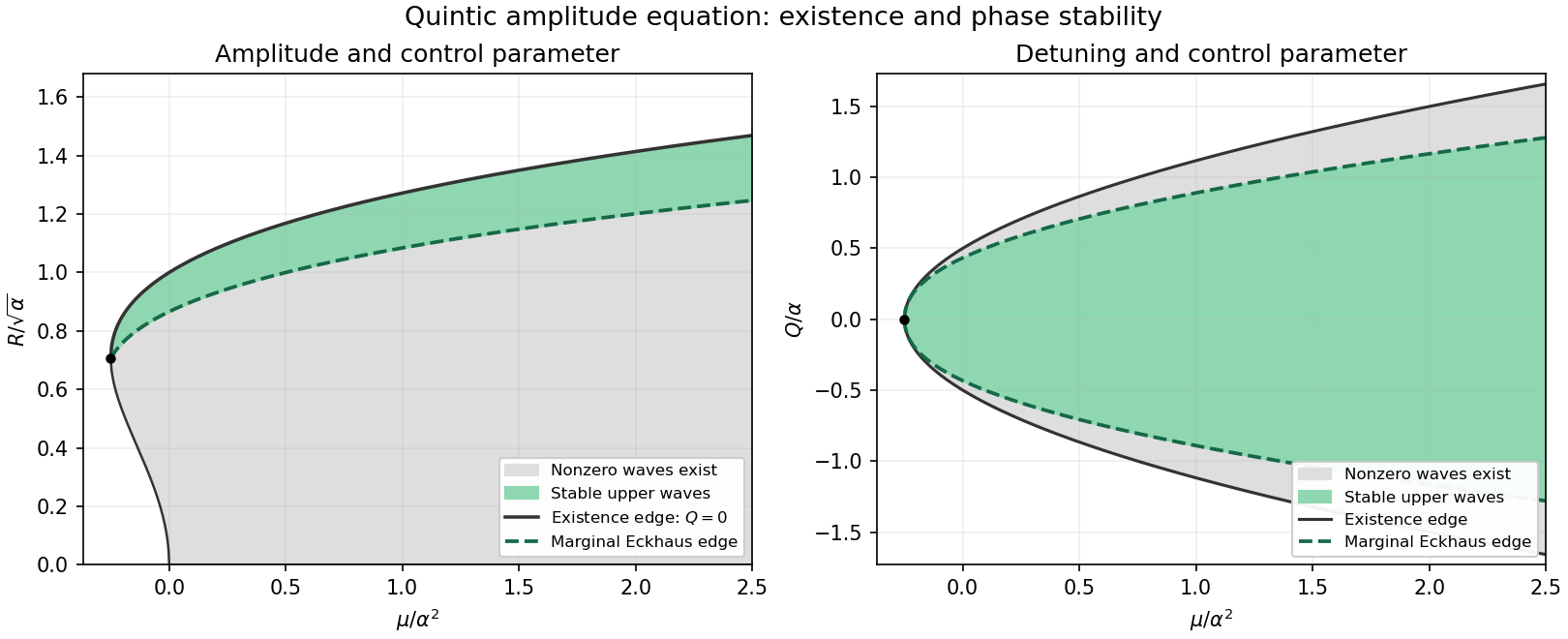
The requested regions can be expressed without eliminating . In the plane, nonzero waves exist wherever . The robust stable part isThe left boundary is the zero-detuning wave ; the right boundary is the marginal Eckhaus curve. Both meet at . At fixed , an equivalent description iswith the lower endpoint added if only marginal linear stability is required.
In the plane, eliminate from the marginal condition. It gives , henceThe equality curve is the marginal boundary; the existence boundary is . They touch at but separate for nonzero detuning, leaving an unstable wave band. Equivalently, for fixed the robust stable interval isThe stable amplitude is the upper root throughout this interval. The sketch uses scaled coordinates , so it applies to every fixed positive . Green denotes stable nonzero waves; the marginal curves form its boundaries, while the surrounding gray region contains existing but unstable nonzero waves.
Pinned article: Introduction to the OurBigBook Project
Welcome to the OurBigBook Project! Our goal is to create the perfect publishing platform for STEM subjects, and get university-level students to write the best free STEM tutorials ever.
Everyone is welcome to create an account and play with the site: ourbigbook.com/go/register. We belive that students themselves can write amazing tutorials, but teachers are welcome too. You can write about anything you want, it doesn't have to be STEM or even educational. Silly test content is very welcome and you won't be penalized in any way. Just keep it legal!
Intro to OurBigBook
. Source. We have two killer features:
- topics: topics group articles by different users with the same title, e.g. here is the topic for the "Fundamental Theorem of Calculus" ourbigbook.com/go/topic/fundamental-theorem-of-calculusArticles of different users are sorted by upvote within each article page. This feature is a bit like:
- a Wikipedia where each user can have their own version of each article
- a Q&A website like Stack Overflow, where multiple people can give their views on a given topic, and the best ones are sorted by upvote. Except you don't need to wait for someone to ask first, and any topic goes, no matter how narrow or broad
This feature makes it possible for readers to find better explanations of any topic created by other writers. And it allows writers to create an explanation in a place that readers might actually find it.
Figure 1. Screenshot of the "Derivative" topic page. View it live at: ourbigbook.com/go/topic/derivativeVideo 2. OurBigBook Web topics demo. Source. - local editing: you can store all your personal knowledge base content locally in a plaintext markup format that can be edited locally and published either:This way you can be sure that even if OurBigBook.com were to go down one day (which we have no plans to do as it is quite cheap to host!), your content will still be perfectly readable as a static site.
- to OurBigBook.com to get awesome multi-user features like topics and likes
- as HTML files to a static website, which you can host yourself for free on many external providers like GitHub Pages, and remain in full control

Figure 2. You can publish local OurBigBook lightweight markup files to either OurBigBook.com or as a static website.
Figure 3. Visual Studio Code extension installation.
Figure 5. . You can also edit articles on the Web editor without installing anything locally. Video 3. Edit locally and publish demo. Source. This shows editing OurBigBook Markup and publishing it using the Visual Studio Code extension. 
- Infinitely deep tables of contents:




All our software is open source and hosted at: github.com/ourbigbook/ourbigbook
Further documentation can be found at: docs.ourbigbook.com
Feel free to reach our to us for any help or suggestions: docs.ourbigbook.com/#contact