Topics (384k) Articles (398k) Users (410) Discussions (242) Comments (383) Files (13k) New article

Radio triangulation estimates a radio transmitter's position by combining directions measured from different known locations. Each radio direction finding observation supplies a bearing line, with the forward direction selecting a ray. Their intersection gives an ideal position estimate. This is one method of radio tracking; detecting a signal at one station does not determine its distance.[ref]
What is Radio Telemetry? by the Smithsonian Migratory Bird Center. Triangulation: directions obtained at separate receiving locations
For two stations at and in a horizontal Cartesian coordinate system, let their bearings make angles and from the positive horizontal axis. Away from vertical bearings, their lines satisfy and . Solving givesFor , and , the result is . The intersection must also lie in each observed forward direction; intersecting the infinite lines alone is insufficient.
The denominator exposes a limitation: nearly parallel bearings can make the position estimate highly sensitive to angular error. Observations taken at different times can also refer to different target positions. More stations allow consistency checks or a fitted estimate when noisy lines do not meet at a point. Smithsonian bird-tracking researchers use this combination of bearings to locate animals without needing continuous visual contact.[ref]
What is Radio Telemetry? by the Smithsonian Migratory Bird Center. Radio-tag localization methods and limits of local tracking
Spatially averaged radiant exposure is the received radiant energy divided by the specified receiving area. For a patch and local radiant exposure ,Both local and averaged values have units , but the average need not equal the local maximum. The radiant exposure definition uses incident energy and the receiving surface's area.[ref]
For an original unequal-area example, let one region receive a uniform , and a neighbouring region receive . They receive and respectively. The average over the combined patch is thereforeThe unweighted average of the two listed exposure values would be , which is wrong for these unequal areas. The area weighting of radiant exposure gives the larger region three times the influence. The actual peak remains in the stipulated piecewise-uniform model.
A receiver integrating all incident energy over the complete patch can determine ; division by its known collecting area then gives the average. That measurement alone cannot identify the peak or reconstruct the spatial distribution. Subdivision with a characterized spatial response supplies additional information. For a finite aperture intercepting a Gaussian beam, use energy actually entering the aperture, as calculated in radiant exposure of a Gaussian beam, rather than the total energy of the untruncated beam.
The radiant exposure of a Gaussian beam is its time-integrated transverse irradiance. At a fixed plane normal to a circular Gaussian beam, suppose the Gaussian beam radius is unchanged during a pulse and denotes the radius where irradiance is of the on-axis value. With total laser pulse energy ,The primary beam account specifies this radius convention and the corresponding irradiance normalization; the radiant exposure parent derives its time integral.[ref]
Propagation of a Gaussian Beam Through a Thin Lens by Francesco D'Angelo. Gaussian Beam: Definition and Characteristics, equation1 and radius definition
An original aperture example asks how much of that energy a finite receiver collects. Integrating over a centred disk of radius gives the encircled radiant energy of a Gaussian beam:For stipulated , and , the receiver collects only percent, or . Its spatially averaged radiant exposure is about , compared with on-axis . Dividing the total by this receiver's area would count energy that missed it.
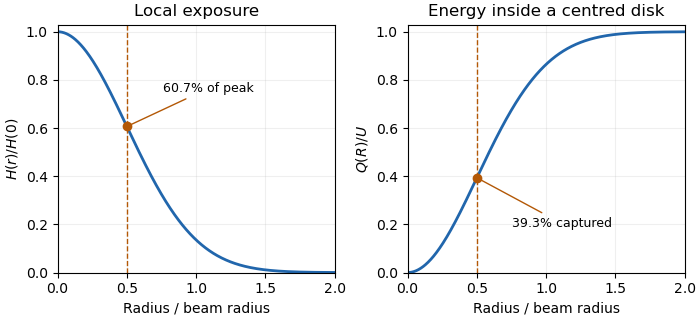
Local Gaussian radiant exposure and cumulative energy capture describe different functions of radius.
Details. To collect a chosen fraction under this ideal model, the centred aperture needs . For95percent, . A possible experimental check measures integrated received energy through several known apertures and compares their ratios. Aperture centring, detector linearity and any profile change during the pulse affect that comparison. A time-varying radius must remain inside the time integral rather than being replaced by an unspecified average radius.
A radiometric energy balance accounts for radiant energy crossing the specified measurement boundary during a specified interval. For a passive optic, suppose the relevant transient has finished, no electromagnetic energy remains stored, and no additional energy source is present. Incident radiation is partitioned into all outgoing radiation and energy transferred to matter. Resolving outgoing paths givesThe channels must be disjoint: a scattering term cannot include energy already counted by a reflection or transmission collector. The definition of radiant energy concerns radiation emitted, transferred or received, so the location and collection geometry belong in each term.[ref]
International Lighting Vocabulary by CIE. Entry17-21-041, definition and note1
For an original example, inject and measure in the transmitted path plus in the specular reflection. Calling the missing absorbed is premature. If a separate collector finds of diffuse outgoing radiation outside those channels, the inferred absorbed energy is only . The uncollected scattering in a radiometric energy balance would otherwise be misidentified as optical absorption.
A physical check compares calibrated incident and outgoing energy readouts while controlling apertures, backgrounds and the observation window. The scattered component may need a different collection geometry from the specular beam. Energy absorbed by matter can remain stored or later leave as heat or radiation; a more general control-volume balance must explicitly include storage, other heat transfer and work. It must not count absorbed energy twice by also treating the same material-energy increase as an independent loss.
The Rabin-Williams scheme is a family of modified Rabin cryptosystem constructions using a modulus with distinct prime numbers and . These congruences make sign and doubling adjustments useful for producing quadratic residues before taking modular square roots. In signature variants, the private integer factorization permits root extraction while the public verification uses squaring.
The arithmetic mechanism can be seen without fixing a full message encoding. For a unit modulo , exactly one of is a quadratic residue modulo both primes: the two signs change both Legendre symbols, while multiplication by changes only one of them. For the toy modulus and , the adjustment has square root , since .
A complete digital signature scheme must additionally specify message hashing or redundancy, the selected root, and how the adjustment is encoded and verified. The congruence calculation alone is not such a scheme. A specific modified-Rabin message-recovery construction is given in the primary handbook, rather than being identical to raw four-root Rabin encryption.[ref]
Handbook of Applied Cryptography by Alfred J. Menezes, Paul C. van Oorschot and Scott A. Vanstone. Section 11.3.4, Fact 11.28 and Algorithms 11.29–11.30; notes to section 11.3 credit Williams
For a single-server queue using first come first served, let be the arrival time of job , its service time, and its departure time. Number jobs in arrival order, with an explicit order for ties. Assume the server works whenever a job is waiting, service is not interrupted, and jobs are neither lost nor dropped. If the server is initially free at time 0 and arrivals are nonnegative, set . ThenThe proof is a scheduling constraint: job cannot start before it arrives or before the preceding job has finished. Under the stated work-conserving rule it starts at the later of those times, then requires more units of time.
Its queueing delay and customer sojourn time are consequentlyFor an original four-job example, use arrivals and service times . The third job follows the second in the tie:The fourth job arrives exactly when the third finishes and therefore has zero queueing delay.
The same recursion also gives a sample-path comparison without assuming a particular arrival or service probability distribution. If every arrival time and service time is increased, and the initial available time is not reduced, induction through the monotone max and addition operations shows that no corresponding departure time decreases. This does not imply that every queueing delay increases: a later arrival can spend less time waiting for the same departure opportunity.
The Quantum Fisher information measures the local sensitivity of a parametrized density matrix . The symmetric logarithmic derivative satisfies , and .
For independent preparations, a locally unbiased estimator obeys under the usual regularity assumptions. For a pure family , . A state with definite acquires only a global phase and has zero information about ; a superposition can have observable relative-phase sensitivity.[ref]
A quantum correlation is a statistical relation among observables of a composite quantum system. For local observables and , a useful diagnostic is . Product states make this expression vanish for every pair of local observables.
Not every correlation in a quantum state is quantum entanglement. The separable mixture gives perfectly correlated computational-basis outcomes but has no entanglement. The pure Bell state has the same outcomes in that basis while retaining coherent relative-phase information detectable in complementary bases. The measurement choices therefore matter when characterizing the kind of correlation present.
A quadrupole stability diagram plots the parameter combinations for which an ideal quadrupole mass analyzer gives bounded transverse ion motion. The useful region is the overlap of stability in both transverse directions: confinement along only one direction still allows loss along the other. The physical selection mechanism is stability in combined static and high-frequency quadrupole electric fields.[ref]
Quadrupole mass analyser in IUPAC Gold Book. Q04971: selected mass-to-charge ratios have stable trajectories; other trajectories are unstable.
Using the potential convention stated in quadrupole mass analyzer, introduce dimensionless time and parametersHere is electric charge, is mass, describes geometry, is drive angular frequency, and specify the static and alternating potentials. The transverse equations becomeThese are Mathieu equations. In the convention , the first equation has ; quoting a diagram requires checking this sign and the potential's numerical convention.
A useful limiting test is , . The equation oscillates, but the equation has exponentially growing solutions. Static focusing alone therefore fails to provide a stable overlap. Periodic focusing changes this conclusion; its stability regions cannot be read off from the force at one instant.
At fixed positive , changing mass-to-charge ratio moves a point along a ray with . Doubling halves both coordinates. Doubling both applied potentials moves the same ion twice as far along that ray. These scaling relations explain how scanning the potentials selects successive mass-to-charge ratios. A stable region is a property of the ideal differential equations; finite rod length, entrance conditions and field imperfections still determine actual transmission and mass resolving power.
The Witt index of a nondegenerate quadratic form on a finite-dimensional vector space is the largest dimension of a totally isotropic subspace: a linear subspace for which for every . In characteristic different from two, the Witt decomposition writeswhere is a hyperbolic plane of a quadratic form, is an anisotropic quadratic form, and is the Witt index. The anisotropic part has no nonzero vector on which the form vanishes.[ref]
For the real form , the subspace spanned by and is totally isotropic. Projection onto the two negative coordinates is injective on any totally isotropic subspace, giving the matching upper bound two. More generally, a real form of signature has Witt index .
The base field matters: has index zero over but index one over , using the line spanned by . In characteristic two, vanishing of the associated polar form on alone is insufficient; the condition remains . Over a finite field, the two nondegenerate types in dimension have Witt indices and .[ref]
The geometry of orthogonal groups over finite fields by Akihiro Munemasa. section 2, definition of Witt index and Theorem 2.11
For a finite-dimensional nonsingular quadratic form over a field of characteristic different from two, a Witt decomposition is an orthogonal splittingwhere is a hyperbolic plane of a quadratic form and is an anisotropic quadratic form. The integer is the Witt index. Both and the isometry class of the anisotropic part are determined by , although the particular subspaces realizing the splitting need not be unique.[ref]
Over , take . Set , and . Thenso . The one-dimensional remainder is anisotropic and the Witt index is one. This is an isometry of quadratic spaces, stronger than merely expressing the underlying vector space as a direct sum.
The construction starts from an isotropic vector, finds a partner with nonzero polar pairing, and splits off the hyperbolic plane they generate. Repeating the process ends when no nonzero isotropic vector remains. The decomposition makes the isotropic directions and the residual arithmetic obstruction visible separately.
A quadratic form over a field is an anisotropic quadratic form if forces . An isotropic quadratic form instead has a nonzero zero vector. This is a property of the form together with its coefficient field, rather than just the displayed polynomial.[ref]
Introduction to quadratic forms by Bill Casselman. Section 2, isotropic and anisotropic vectors, printed page 5
For example, is anisotropic over . If a nonzero rational solution had , then too; otherwise would be a rational square root of two. Over , however, is a nonzero zero vector. The coordinate change , gives , a hyperbolic plane of a quadratic form.
This example also separates anisotropy from positive definiteness: the rational form takes the positive value and the negative value , despite having no nonzero rational zero. In a Witt decomposition, an anisotropic remainder is what remains after all hyperbolic planes have been split off. Its Witt index is zero. In characteristic two, one must test vanishing of the quadratic form itself; properties of the associated polar bilinear form alone do not supply the same test.
Pinned article: Introduction to the OurBigBook Project
Welcome to the OurBigBook Project! Our goal is to create the perfect publishing platform for STEM subjects, and get university-level students to write the best free STEM tutorials ever.
Everyone is welcome to create an account and play with the site: ourbigbook.com/go/register. We belive that students themselves can write amazing tutorials, but teachers are welcome too. You can write about anything you want, it doesn't have to be STEM or even educational. Silly test content is very welcome and you won't be penalized in any way. Just keep it legal!
Intro to OurBigBook
. Source. We have two killer features:
- topics: topics group articles by different users with the same title, e.g. here is the topic for the "Fundamental Theorem of Calculus" ourbigbook.com/go/topic/fundamental-theorem-of-calculusArticles of different users are sorted by upvote within each article page. This feature is a bit like:
- a Wikipedia where each user can have their own version of each article
- a Q&A website like Stack Overflow, where multiple people can give their views on a given topic, and the best ones are sorted by upvote. Except you don't need to wait for someone to ask first, and any topic goes, no matter how narrow or broad
This feature makes it possible for readers to find better explanations of any topic created by other writers. And it allows writers to create an explanation in a place that readers might actually find it.
Figure 1. Screenshot of the "Derivative" topic page. View it live at: ourbigbook.com/go/topic/derivativeVideo 2. OurBigBook Web topics demo. Source. - local editing: you can store all your personal knowledge base content locally in a plaintext markup format that can be edited locally and published either:This way you can be sure that even if OurBigBook.com were to go down one day (which we have no plans to do as it is quite cheap to host!), your content will still be perfectly readable as a static site.
- to OurBigBook.com to get awesome multi-user features like topics and likes
- as HTML files to a static website, which you can host yourself for free on many external providers like GitHub Pages, and remain in full control

Figure 2. You can publish local OurBigBook lightweight markup files to either OurBigBook.com or as a static website.
Figure 3. Visual Studio Code extension installation.
Figure 5. . You can also edit articles on the Web editor without installing anything locally. Video 3. Edit locally and publish demo. Source. This shows editing OurBigBook Markup and publishing it using the Visual Studio Code extension. 
- Infinitely deep tables of contents:



All our software is open source and hosted at: github.com/ourbigbook/ourbigbook
Further documentation can be found at: docs.ourbigbook.com
Feel free to reach our to us for any help or suggestions: docs.ourbigbook.com/#contact