Topics (384k) Articles (398k) Users (410) Discussions (242) Comments (383) Files (13k) New article

The real Schur form of a real square matrix is , where is orthogonal and is upper quasi-triangular. Its diagonal consists of one-by-one blocks for real eigenvalues and two-by-two blocks for complex-conjugate pairs.
The rotation generator already forms one two-by-two block with eigenvalues . No real upper-triangular matrix can have those eigenvalues, because its diagonal entries would all be real. Real Schur form therefore permits real arithmetic without pretending every eigenvalue is real. Its orthogonal transformations are also preferable numerically to using a potentially ill-conditioned eigenvector matrix.[ref]
Eigenvalues and Schur Forms in the LAPACK Users' Guide. Ordinary Schur factorization and real diagonal blocks
Pyridoxine phosphate is the 5′-phosphate derivative of pyridoxine, one of the forms of Vitamin B6. Attaching a phosphate group and changing an alcohol group into an aldehyde are different chemical modifications. Pyridoxine phosphate still differs from pyridoxal phosphate, the form used as a coenzyme in many reactions.[ref]
Vitamin B6 Fact Sheet for Health Professionals by the Office of Dietary Supplements. Introduction: six vitamin B6 forms and their phosphorylated derivatives
An important connection is the oxidation of pyridoxine phosphate by pyridoxal 5'-phosphate synthase. The official reaction isHere oxygen accepts the reducing equivalents, producing hydrogen peroxide; the phosphate group is retained. The enzyme contains flavin mononucleotide.[ref]
For a constructed material-balance example, complete conversion of 4 micromoles of pyridoxine phosphate through this reaction consumes 4 micromoles of oxygen and forms 4 micromoles each of pyridoxal phosphate and hydrogen peroxide. There is no net release of free phosphate in that reaction. Measuring only total phosphorus would therefore miss the conversion: the substrate and product each retain one phosphorus atom. A measurement that distinguishes their functional groups can answer a question that elemental accounting cannot.
Pyridoxamine phosphate usually denotes pyridoxamine 5'-phosphate, the phosphate ester of the position-5 hydroxymethyl group of pyridoxamine. Its neutral-form molecular formula is . It is an active Vitamin B6 coenzyme form, chemically distinct from both free pyridoxamine and pyridoxal phosphate.[ref][ref]
Vitamin B6 Fact Sheet for Health Professionals by the Office of Dietary Supplements. Introduction, active PLP and PMP coenzyme forms
A concrete reaction distinguishes the two phosphorylated forms. Pyridoxal 5'-phosphate synthase can oxidatively convert pyridoxamine phosphate into pyridoxal phosphate, producing Ammonia and hydrogen peroxide while consuming water and oxygen.[ref] The transformation changes the aminomethyl group into an aldehyde group while retaining the phosphate ester.
For an ideal conversion by this reaction, one micromole each of Ammonia and hydrogen peroxide is produced. A peroxide assay can consequently report a coupled reaction signal, but identifying the B6 product remains a separate analytical question. A peroxide-producing impurity could mimic that signal without making the intended coenzyme.
Separating detector noise from pulse-energy variance estimates source variability using a model of the readout's own fluctuations. In energy-calibrated units, write . The exact identity isOnly when the covariance vanishes can a separately estimated noise variance be subtracted directly. Covariance terms are part of measurement-model uncertainty propagation, rather than an optional correction.[ref]
For an original independent-noise example, suppose the observed energy standard deviation is and a matched noise-only measurement gives . The inferred source standard deviation is , not . The source contributes of the observed variance in this stipulated model.
A noise-only record should use comparable gain, integration gate and reset conditions. Background subtraction removes an estimated mean, not the random variance remaining around it. Amplifier clipping, unmatched integrator reset or signal-dependent detector noise can invalidate an additive independent-noise model. A negative variance difference is not a physical negative source variance; it can indicate estimation uncertainty or mismatched assumptions.
Splitting pulses between two independently characterized readouts can provide a two-channel covariance estimate of pulse-energy variance under additional noise assumptions. Shared electronics noise and common drift must still be assessed; independence cannot be established just by using two detectors.
Nonuniqueness of pulse energy at fixed peak power and FWHM means that those two measurements do not determine the integral of an otherwise unspecified power profile. The pulse energy shape factor gives a rectangular/exponential counterexample. A stronger original construction shows there is no finite universal upper bound without restrictions on lower-level tails.
Fix , power FWHM , and . Choose any . Let the power equal for , equal for , and zero afterward. The optical pulse pedestal is part of the stipulated signal, not an unrelated background. Its level stays below half maximum, so the peak and FWHM remain unchanged, butWith and , the energy is , compared with for the pedestal-free rectangle. Increasing finite gives unbounded pulse energy at fixed peak and FWHM across this family of finite-duration ideal profiles.
This is an identifiability result, not a claim that a particular laser has arbitrarily long tails. The primary source definition of power-FWHM fixes a threshold width, not the integrated energy below that threshold.[ref]
Plane wave and beam source - Simulation object in Ansys Optics documentation. PULSELENGTH definition
A measured full profile, a justified shape family or additional tail-duration bounds supply information that peak and FWHM omit.Baseline-drift bias in pulse-energy integration is the systematic energy error caused by using an inaccurate baseline over the integration gate. Relative to the true signal energy in the same gate,This error is separate from energy excluded by the gate. Historical NIST measurements bracketed each run with baseline observations and subtracted their average to compensate background and thermal drift.[ref]
Calibration Service for Low-level Pulsed-Laser Radiometers at 1.06 µm: Pulse Energy and Peak Power by Rodney W. Leonhardt. §3.5; §7.2, Type B component4, Leakage Effect
An original curvature example shows a limit of endpoint bracketing. On , suppose . Both endpoint baselines equal , so their average and the straight interpolation between them coincide. However, the true integrated baseline is . Subtracting the endpoint level over the whole gate therefore givesFor a gate whose endpoints are above its midpoint baseline, this bias is . A true gated signal energy of would be reported as under these assumptions.
Thus quadratic baseline curvature in gated energy integration survives a correction that is exact for a linear baseline. For fixed curvature, the error grows with the cube of gate duration. Additional pulse-free samples can test the baseline model, but pulse tails in those samples can themselves corrupt the estimate. Pulse energy baseline correction supplies the broader measurement context.
Pseudomonas syringae is a species of bacteria in Pseudomonas, important in the study of interactions between plants and their associated microorganisms. Its nomenclatural type strain is deposited under identifiers including ATCC19310 and NCPPB281. Such collection identifiers locate reference material; they are not interchangeable with every experimental bacterial strain assigned to the species.[ref]
A 2011 experiment used the strain reported as Pseudomonas syringae pv. tomato DC3000 to challenge Arabidopsis thaliana. Plants were grown with or without candidate bacterial colonists. Some Sphingomonas isolates reduced both pathogen growth and disease symptoms, whereas the tested Methylobacterium strains did not show that protective effect. The experiment asked whether prior colonization changed an observed disease outcome, rather than merely whether both organisms could be detected on a leaf.[ref]
Pathogen population and host damage are distinct readouts. In an invented normalized-count example, versus colony-forming units per gram of leaf differs tenfold, or by one base-ten logarithmic unit. That calculation alone supplies neither a disease-severity score nor proof of a particular protective mechanism. Host, strain identity and measurement conditions remain part of the interpretation.
A homotrimer is a protein trimer containing three copies of the same protein subunit type. “Homo” specifies composition; “trimer” specifies a total of three subunits. A homotrimer need not have perfectly identical instantaneous conformations or ligand occupancies at all three copies.
Polynucleotide phosphorylase provides a functional example. Its three repeated subunits form a ring around the polynucleotide phosphorylase central channel. Cryo-electron microscopy of the mycobacterial enzyme resolved that ring and RNA near a catalytic site, connecting an oligomeric structure with an RNA-processing mechanism.[ref]
Structure and mechanism of Mycobacterium smegmatis polynucleotide phosphorylase by Mihaela-Carmen Unciuleac and others. Abstract and Figure1, homotrimeric core; RNA-bound reconstructions
For an original conservation example, let be an unassembled chain and the assembled homotrimer, with no other forms present:A total chain concentration of can yield at most trimers. If half the chains remain unassembled, only trimers form. Reporting concentration in chains or in complexes therefore changes the numerical value even for the same preparation.
A heterotrimer is a protein trimer containing more than one type of protein subunit. It may have composition or , for example; the total number of subunits is three in either case. This distinguishes it from a homotrimer, whose three subunits have the same type.
A heterotrimeric G protein illustrates the arrangement, with distinct , and subunits. A structural inhibitor study crystallized an engineered complex and separately measured nucleotide binding and release. Such experiments distinguish the composition of the assembled complex from the chemical activity of one of its components.[ref]
Structural basis for the specific inhibition of heterotrimeric Gq protein by a small molecule by Akiyuki Nishimura and others. Materials and Methods, protein preparation, crystallization and nucleotide assays
For an original assembly bound, start with of , of and of , allowing only complexes. At most complexes can form, leaving at least of and of outside them. Adding more alone cannot overcome the shortage of . Actual assembly may be lower because of incomplete binding or competing complexes.
A protein subunit is an individual polypeptide component of a protein complex. The number of protein subunits counts chain copies, whereas the number of subunit types counts distinct kinds of chain. An assembly has four protein subunits of two types. A protein domain is a region within a chain and need not be a separate protein subunit; the arrangement of several chains belongs to protein quaternary structure.
The alpha/beta tubulin heterodimer illustrates the distinction: it contains two related but different polypeptides, not two domains cut out of one chain. The 1998 electron-crystallographic model resolved the alpha/beta architecture at angstrom resolution, using zinc-induced tubulin sheets.[ref]
Structure of the alpha beta tubulin dimer by E. Nogales and others. Abstract and PDB entry 1TUB: distinct alpha and beta chains and electron-crystallographic method.
Subunit counting can also become an optical experiment. In total internal reflection fluorescence microscopy, tagged membrane proteins can be observed as isolated fluorescent spots; successive photobleaching steps reveal individual fluorescent tags disappearing. Subunit counting in membrane-bound proteins by Maximilian H. Ulbrich and Ehud Y. Isacoff used this approach on membrane proteins expressed in frog oocytes. For NR1/NR3B receptor assemblies, tagging one component type mainly gave two steps, while tagging both gave four, supporting a two-plus-two arrangement.[ref]
Subunit counting in membrane-bound proteins by Maximilian H. Ulbrich and Ehud Y. Isacoff. Figures 1–2 and results on NR1/NR3B stoichiometry.
A count of visible steps need not equal the true number of protein subunits: some tags fail to fluoresce, and two tags may bleach too close together to resolve. The experiment therefore combines step counts with a model of labeling and detection, rather than interpreting every two-step trace as proof of a two-chain protein complex.[ref]
Subunit counting in membrane-bound proteins by Maximilian H. Ulbrich and Ehud Y. Isacoff. Discussion of fluorescent-tag probability, approximately 80%, and binomial interpretation of bleaching-step distributions.
In protein chemistry, a heterodimer is an assembly of two different protein subunits, conventionally written . A homodimer has two copies of the same subunit type, . Different types can have similar protein folds and nearly equal molecular masses; “different” refers to molecular identity, not simply size or shape. An protein complex contains two types but four chains, so it is not itself a heterodimer.
The alpha/beta tubulin heterodimer is the repeating building block of a microtubule. The alpha and beta protein subunits have similar folds but distinct sequences and nucleotide environments. Their structural relationship was resolved by electron crystallography of zinc-induced tubulin sheets: the 1998 model reached angstrom resolution. This is a concrete example of a two-chain protein quaternary structure, rather than the protein tertiary structure of a single chain.[ref]
Structure of the alpha beta tubulin dimer by E. Nogales and others. Abstract: approximately 40% alpha/beta sequence identity, closely similar folds, distinct nucleotide-binding sites and experimental method.
Stoichiometry gives a useful upper bound. If an idealized mixture contains of and of , and only can assemble, at most of heterodimer can form; at least of remains outside . The actual amount also depends on binding equilibrium and experimental conditions: chain counting alone does not guarantee complete association.
A homodimer is a protein complex containing two copies of the same protein subunit type, conventionally written . A heterodimer instead contains two different types, . Identical subunit type does not require the copies to occupy identical conformations or environments in every instant of the complex's motion.
Assembly is part of protein quaternary structure, rather than a claim that the two chains have become one longer polypeptide. If each subunit contains 100 amino acid residues, the homodimer contains 200 residues across two chains. Association alone need not add a peptide bond between them.
For reversible association , a concentration-form dissociation constant isThe second equation counts subunit equivalents. For and , : half the subunit copies reside in dimers, even though dimers comprise only one third of the separate molecular particles. The written uses the usual macroscopic concentration convention.
HIV-1 protease supplies an experimentally important example. Recombinant enzyme had reported molecular masses of approximately 11,000 under denaturing conditions and 22,000 under nondenaturing conditions; chemical crosslinking provided additional evidence consistent with an active two-subunit enzyme. Comparing several measurements was more informative than assigning a homodimer solely from an apparent mass in one assay.[ref]
Human immunodeficiency virus 1 protease expressed in Escherichia coli behaves as a dimeric aspartic protease by T. D. Meek and others. Abstract: molecular-mass comparison, chemical crosslinking and protease activity.
A nucleoprotein complex is an assembly containing both nucleic acid and protein components. The nucleic acid can be DNA or RNA, and its spatial arrangement and contacts with the proteins are part of the structure. A mixture that merely contains both kinds of molecule is not automatically one associated complex.
The nucleosome core particle is a concrete DNA–protein example. The1997 structure reported by Karolin Luger and colleagues contains146 base pairs of DNA wrapped around a histone octamer. It shows both protein–protein and protein–DNA contacts. Counting the components and mapping their contacts answer different questions: eight histone molecules do not imply eight identical DNA-binding environments.[ref]
A bacterial small ribosomal subunit provides an RNA–protein example. Its 16S ribosomal RNA and ribosomal proteins form an organized assembly used in translation. The2000 crystal structure links the RNA/protein arrangement to earlier biochemical observations, showing why the nucleic acid is a structural participant rather than merely something carried inside a protein shell.[ref]
Structure of the 30S ribosomal subunit by B. T. Wimberly and others. Abstract:30S nucleoprotein structure and RNA–protein architecture
An experiment must also distinguish association from coincidental presence. Co-purification can suggest a complex, while a resolved structure can identify actual contacts; neither an ingredient list nor a bulk protein measurement alone specifies the architecture.
A refutation of a collection of logical assumptions is a derivation of a contradiction from them. To prove a logical formula by refutation in classical propositional logic, add its negation to the assumptions and derive falsity. The correctness of this inference follows from the rules of the chosen proof system.
For example, the clauses , and have a resolution refutation: the first two resolve to , and with yields the empty clause. No truth assignment satisfies the three original clauses. This distinguishes the semantic claim of unsatisfiability from a syntactic certificate establishing it. In automated proving, producing a refutation is useful because another program can check the individual inference steps without repeating the search.
A proficiency-test z-prime score modifies a proficiency-test z-score to include uncertainty of the assigned value in proficiency testing:Here is the standard deviation for proficiency assessment, and is the assigned value's standard uncertainty. The latter describes uncertainty in the comparator, not the participant's reported uncertainty.[ref]
An original example gives units, units and units. The ordinary score is 3; the modified denominator is units and . Under the guide's common interpretation, the first reaches the action boundary and the second lies in the warning interval. The change reflects benchmark uncertainty, not a change in the measured result.
The effect can be separated algebraically. Put . ThenWhen , the magnitude is about 0.958 times the ordinary score. The guide treats a contribution below as negligible for ordinary score interpretation. Conversely, when becomes very large, the modified score tends toward zero for any fixed deviation. A weak benchmark can therefore make a discrepancy difficult to interpret; it cannot make a measurement intrinsically accurate.[ref]
Selection, Use and Interpretation of Proficiency Testing (PT) Schemes by Brian Brookman and Ian Mann. §7.2.6, uncertainty criterion; §7.2.4, cautions on z-prime interpretation
Do not replace the assessment scale with the laboratory's uncertainty and still call the result this score. An uncertainty-normalized compatibility calculation asks a different question. Likewise, if the assigned value uses the participant's own result, participant influence on a consensus assigned value creates dependence that must be understood before interpreting the score as an independent check.
The scheme should state its score and benchmark treatment in advance. When assigned-value uncertainty is too large, options include improving the reference assignment or explicitly reporting its limitations. Enlarging a denominator after seeing an inconvenient result does not supply new measurement evidence.
Differences between supplied proficiency-test items can contribute to a proficiency-test z-score even when the laboratory's own measurement procedure has zero systematic error. Model the result from laboratory aswhere is an independently established batch target, is the supplied unit's deviation, is a fixed laboratory systematic error, and is analytical variation. Assume centered independent and , with variances and , and treat the assigned value in proficiency testing as exactly for this model. Then the proficiency-test z-score satisfieswhere is the standard deviation for proficiency assessment. A large deviation cannot be attributed to from the score alone. The primary guide requires item reference material homogeneity and reference material stability to remain appropriate when a stricter assessment scale is selected.[ref]
Selection, Use and Interpretation of Proficiency Testing (PT) Schemes by Brian Brookman and Ian Mann. §8.2.3, printed p. 21, smaller assessment scales and item suitability
A homogeneity study with replicated test portions can separate two variance components. Select units and measure independently drawn portions from each using one verification method, with measurement order randomized across units. Under the random effect model , independent equal-variance within-unit errors give the one-way analysis of variance mean squaresTheir expectations are and . A method-of-moments variance component estimate is therefore . Here the within-unit component is treated as analytical variation; variation between portions of the same unit would also enter it unless separated by further measurements. Clipping a negative estimate to zero enforces a nonnegative variance component; it introduces boundary bias and does not establish perfect material uniformity.
For an original arithmetic example, four units yield the following paired mass concentration readings, in :The overall arithmetic mean is . These chosen data give , and , with squared concentration units. Suppose a participant also has analytical variance and the assessment scale is . The stipulated unbiased score then has standard deviation , despite the absence of a laboratory systematic error in the model.
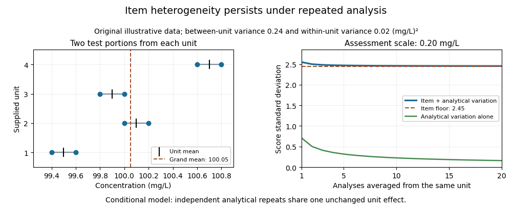
Averaging independent analyses from the same unit changes the analytical contribution to but retains its unit effect:For the chosen numbers, the score's standard deviation approaches as increases. Repeatedly reading one aliquot may reduce an even narrower instrumental contribution. Sampling independently supplied units addresses a different source of variation.
This is an explanatory measurement model, not a prescribed proficiency-testing acceptance rule. Its variance components require evidence about portion size, preparation and measurement conditions. Instrumental drift confounded with unit order, changing material, correlated errors or an uncertain consensus benchmark require additional terms and an appropriate design. The provider's homogeneity evidence is essential to interpreting the score; a smaller numerical scoring denominator does not improve the items.
The Horvitz-Thompson estimator estimates a finite population total by expanding each observed unit's contribution by the reciprocal of its inclusion probability. D. G. Horvitz and D. J. Thompson introduced the general unequal-probability construction in 1952.[ref]
A Generalization of Sampling Without Replacement From a Finite Universe by D. G. Horvitz and D. J. Thompson. Original publication, Journal of the American Statistical Association 47(260), pp. 663–685, December 1952
Let be fixed values attached to labelled population units. A sampling design selects a random subset , with known inclusion probabilities . Thenwhere is the inclusion indicator. This is inverse probability weighting for a finite population.[ref]
Unequal Probability Sampling in Penn State STAT 506. Lesson 3, Definition 3.2, Horvitz–Thompson estimator
Its expected value is immediatelyThe subscript emphasizes design-based inference: the fixed values are not assumed to follow a probability model; the sample-selection mechanism supplies the randomness. The inclusion indicators need not be independent. Dividing by known gives an unbiased estimator of the finite population mean.For an original exact example, use values and choose samples , , with probabilities , respectively. The inclusion probabilities are . The corresponding estimates of the total are , andSimply multiplying each sample mean by three instead gives totals , with expected value . Equal treatment of the observed values ignores the unequal chances of observing them.
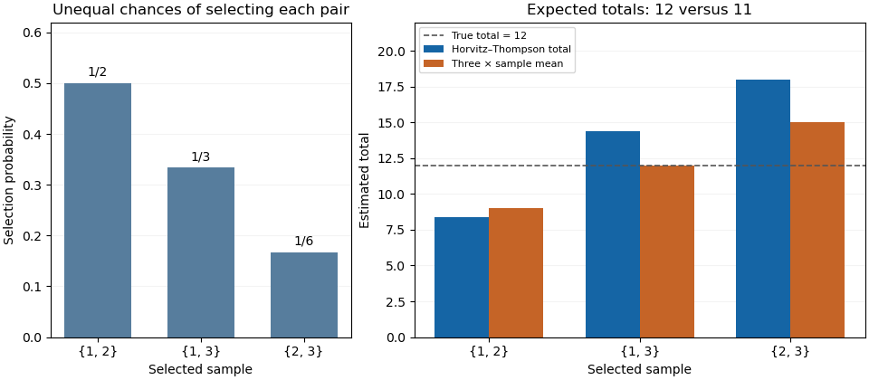
Inverse-inclusion weighting corrects the expected total in an unequal-probability sample
. Original exact enumeration of three possible two-unit samples from values 2, 4 and 6. The left panel shows their selection probabilities; the right compares the Horvitz-Thompson total with three times the sample mean. The population total is 12. Details.The sampling variance depends on pair information. Put , including . Bilinearity of covariance givesFor the three-unit design it is , found directly from . Thus an unbiased estimator need not give a nearly correct total in each sample.
With pairwise inclusion positivity, the same expansion device applied to pairs constructs the Horvitz-Thompson variance estimator:Its expected value equals the preceding population sum because . In the worked design its three possible values are , whose probability-weighted average is . This particular unbiased estimator of variance can therefore be negative for an individual sample. Its expected value identity is a statement about repeated selection.
If , an arbitrary unobserved cannot contribute to an unbiased total estimate. If a distinct pair has , its product cannot be recovered by the pair-expansion argument. Finally, dividing the weighted sum by the random sum of its inverse-probability weights changes the estimator into a ratio; the indicator proof above no longer establishes that this ratio is an unbiased estimator. The known population size and the actual sampling design are part of the result.
A sampling design specifies a probability distribution over the possible samples from a defined population:For sampling distinct labelled units, is a subset of the population. The design includes the selection mechanism, not merely the final sample size. A procedure with repeated draws can instead require a distribution over ordered sequences; the resulting inclusion probabilities concern whether a label appears at least once.
The design determines inclusion probabilities and joint inclusion probabilities throughThese connect the physical sampling procedure to the Horvitz-Thompson estimator and its sampling variance.[ref]
A Generalization of Sampling Without Replacement From a Finite Universe by D. G. Horvitz and D. J. Thompson. 1952, general unequal-probability sampling without replacement
An original comparison uses four fixed values and selects two units. Under simple random sampling, every one of the six pairs has probability . Each , so the Horvitz-Thompson estimator is twice the selected sum. It takes values with probabilities . Its expected value is the true finite population total , and its variance isA second design chooses only or , each with probability . It has the same sample size and the same individual inclusion probabilities, but the estimator is now or , giving variance . Pair selection matters even when individual representation agrees.
A third design chooses uniformly among the four pairs containing one label from each of those two groups. Its total estimate is always for this particular population. This illustrates the potential gain from stratified sampling when groups correspond to relevant variation, not a claim that the third design dominates for every possible population. A reproducible design records the eligible labels and actual random selection rule before interpreting the observed sample.
Design-based inference evaluates an estimator by the random mechanism selecting a sample from a fixed finite population. Population values are held fixed; the selected subset is random under a known sampling design . ThusThe subscript identifies the source of randomness. An unbiased estimator of a finite population total has for each eligible fixed population. The unequal-probability total developed by D. G. Horvitz and D. J. Thompson is a central example.[ref]
A Generalization of Sampling Without Replacement From a Finite Universe by D. G. Horvitz and D. J. Thompson. 1952, unequal-probability sampling and unbiased finite-universe estimation
For an original example, let the fixed population values be and sample one label uniformly. Every inclusion probability is , so the Horvitz-Thompson estimator is . Its three equally probable values are , while the actual total is . Consequently,The estimator is unbiased even though none of its possible estimates equals the target. Unbiasedness describes averaging across the sampling design, rather than guaranteed accuracy in an individual sample.
A confidence interval with design-based coverage must likewise succeed at its stated rate across repeated selections under the specified design. That property requires a justified construction; unbiasedness of a point estimate alone supplies no coverage guarantee. Repeating a convenient calculation on the same selected units does not reproduce the selection process. Assumptions about measurement error or missing responses must also be stated separately, since knowledge of the original selection probabilities alone does not repair those later stages.
A finite population total adds a specified numerical value over every labelled unit in a fixed, finite population :The target must specify both the population and the measured variable. It may be a total inventory mass, the total number of employees across establishments, or the sum of a binary property. If , the total counts units having the property; it is not automatically the population size . A finite population mean is , when is known and positive.
An original inventory has four containers holding of a material. The total is and the finite population mean is per container. Giving every container the same mass fraction of an analyte is a separate assumption: the total analyte mass instead requires summing each container's mass multiplied by its own mass fraction. The target follows the physical quantity being added.
When only a sample is observed, the unweighted sample sum is generally not an unbiased estimator of . Using inclusion indicators and inclusion probabilities givesIf every , the Horvitz-Thompson estimator instead satisfiesThis is a consequence of the sampling design, without requiring the fixed population values to follow a statistical distribution.[ref]
A Generalization of Sampling Without Replacement From a Finite Universe by D. G. Horvitz and D. J. Thompson. 1952, finite-universe estimation framework, pp.663–685
A full census removes sample-selection variation, but imperfect measurement can still make the recorded sum differ from the intended physical total. Pinned article: Introduction to the OurBigBook Project
Welcome to the OurBigBook Project! Our goal is to create the perfect publishing platform for STEM subjects, and get university-level students to write the best free STEM tutorials ever.
Everyone is welcome to create an account and play with the site: ourbigbook.com/go/register. We belive that students themselves can write amazing tutorials, but teachers are welcome too. You can write about anything you want, it doesn't have to be STEM or even educational. Silly test content is very welcome and you won't be penalized in any way. Just keep it legal!
Intro to OurBigBook
. Source. We have two killer features:
- topics: topics group articles by different users with the same title, e.g. here is the topic for the "Fundamental Theorem of Calculus" ourbigbook.com/go/topic/fundamental-theorem-of-calculusArticles of different users are sorted by upvote within each article page. This feature is a bit like:
- a Wikipedia where each user can have their own version of each article
- a Q&A website like Stack Overflow, where multiple people can give their views on a given topic, and the best ones are sorted by upvote. Except you don't need to wait for someone to ask first, and any topic goes, no matter how narrow or broad
This feature makes it possible for readers to find better explanations of any topic created by other writers. And it allows writers to create an explanation in a place that readers might actually find it.
Figure 1. Screenshot of the "Derivative" topic page. View it live at: ourbigbook.com/go/topic/derivativeVideo 2. OurBigBook Web topics demo. Source. - local editing: you can store all your personal knowledge base content locally in a plaintext markup format that can be edited locally and published either:This way you can be sure that even if OurBigBook.com were to go down one day (which we have no plans to do as it is quite cheap to host!), your content will still be perfectly readable as a static site.
- to OurBigBook.com to get awesome multi-user features like topics and likes
- as HTML files to a static website, which you can host yourself for free on many external providers like GitHub Pages, and remain in full control

Figure 2. You can publish local OurBigBook lightweight markup files to either OurBigBook.com or as a static website.
Figure 3. Visual Studio Code extension installation.
Figure 5. . You can also edit articles on the Web editor without installing anything locally. Video 3. Edit locally and publish demo. Source. This shows editing OurBigBook Markup and publishing it using the Visual Studio Code extension. 
- Infinitely deep tables of contents:




All our software is open source and hosted at: github.com/ourbigbook/ourbigbook
Further documentation can be found at: docs.ourbigbook.com
Feel free to reach our to us for any help or suggestions: docs.ourbigbook.com/#contact