Topics (384k) Articles (398k) Users (410) Discussions (242) Comments (383) Files (13k) New article

A unimodal distribution, under the density or mass-function convention, has probabilities that rise toward one central region and then fall away. For an absolutely continuous probability distribution, this means it has a probability density function that is nondecreasing up to a mode and nonincreasing afterward. This is the single-maximum meaning of unimodality; the chosen density is a one-dimensional quasiconcave function. A plateau of maximizing points is allowed.
For a discrete original example on outcomes0,1,2and3, choose probabilities0.1,0.4,0.4and0.1. The probability mass function rises, has two adjacent maximizing values, then falls. It is unimodal under the weak monotonicity definition despite not having a unique mode. In contrast, separated high-probability regions with a genuine dip between them are not one mode plateau.
Unimodality does not imply symmetry or equality of arithmetic mean, median and mode. For the exponential distribution with density on , , the mode is0, the mean is and the median is . The density decreases from its boundary maximum. The NIST handbook gives the family and these summary characteristics, using a scale parameter reciprocal to this rate parameter.[ref]
Exponential Distribution in the NIST e-Handbook. §1.3.6.6.7, Probability Density Function and summary statistics
Nor is unimodality generally preserved by a mixture distribution. Equal mixing of uniform distributions on and gives density1/2 on those two intervals and zero in between. Each component has a flat unimodal density, while the mixture has separated peaks.
A density is defined only up to changes on sets of measure zero. Thus the distributional statement concerns existence of a representative with the required shape, rather than artificial isolated spikes added to one displayed formula. In higher dimensions, several notions of unimodality are used; one convex-level-set formulation requires convex superlevel sets, as in the quasiconcave function definition.[ref] The shape convention should be specified before extending a one-dimensional conclusion to another setting.
A reliability diagram compares predicted probabilities with observed outcome frequencies to assess probability calibration. For the positive-class version of binary classification, partition observations into bins according to their predicted probabilities . For every nonempty bin, plotwhere is for a positive outcome and otherwise. Agreement places the estimated points near the diagonal . Empty bins have no observed fraction and should not be plotted as zero.[ref]
Probability calibration in the scikit-learn documentation. Section 1.16.1: mean predicted probabilities and fractions of positives
Binning can hide important structure. Consider ten cases each assigned , of which eight are positive, and ten cases each assigned , of which two are positive. Separate bins give and , revealing strong disagreement. Merge all 20 cases into one bin: the mean prediction becomes and the positive fraction is . The single point lies on the diagonal despite the two-group discrepancy.
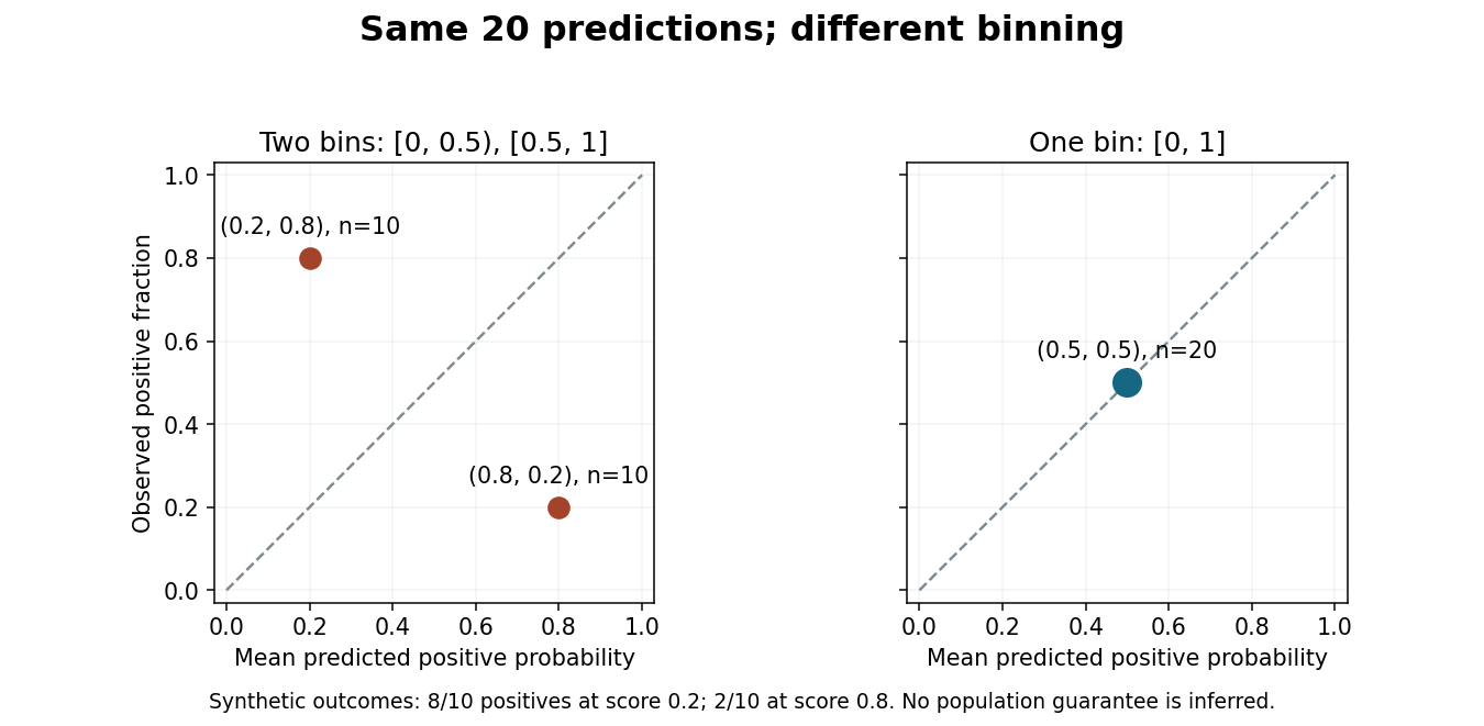
Merging bins can hide disagreement in a reliability diagram.
Original synthetic binary classification example with the same 20 predictions and outcomes in both panels. Points show positive-class frequencies; the diagram does not establish a population guarantee. Details.Report bin definitions and counts, since a point based on ten cases has different sampling uncertainty from one based on thousands. Some classification diagrams instead plot confidence in the selected label against the fraction of correct selections. That convention and the positive-class version answer related but distinct questions, so label the axes and the meaning of the outcome explicitly.[ref]
On Calibration of Modern Neural Networks by Chuan Guo and others. Section 2: selected-label accuracy/confidence convention and limitations of a reliability diagram without bin populations
Temperature scaling is a method of probability calibration that divides a model's neural network logits by one fitted positive scalar before applying the softmax function. The temperature is selected after model training, using labels in a held-out validation set to minimize the negative log-likelihood. It adjusts reported probabilities without retraining all model weights.[ref]
On Calibration of Modern Neural Networks by Chuan Guo and others. §4.2, Eq. (9), scalar temperature and validation negative log likelihood
For class scores and ,For the synthetic two-class scores , the first-class probability isThe selected class remains the first while its reported confidence decreases.
The preservation of the selected class follows directly: dividing by positive preserves every score ordering and equality, and exponentiation is strictly increasing. Thus the set of classes attaining the largest score is unchanged. This concerns ordering between classes within one example; it does not assert preservation of confidence ordering between different examples.
A motivating measurement in the original study compares reliability diagrams for a 110-layer image-classification network. Its reported expected calibration error changes from before calibration to after temperature scaling. This is a result for that experimental setup and binned metric, not a guarantee for every classifier or input distribution.[ref]
On Calibration of Modern Neural Networks by Chuan Guo and others. §5 and Fig. 4, CIFAR-100 ResNet-110 before/after reliability diagrams
Use separate data for fitting the temperature and for final evaluation. One scalar can improve an overall confidence mismatch but cannot represent every class-specific or input-dependent error. The name refers to this probability transformation; no physical temperature is being measured.
Expected calibration error summarizes how reported confidence differs from observed correctness. For top-label statistical classification, the population quantity compares correctness probability conditional on confidence with that confidence. A commonly reported finite-sample estimate groups predictions into confidence intervals and compares the mean confidence and accuracy in each interval.[ref]
On Calibration of Modern Neural Networks by Chuan Guo and others. §2, Eqs. (2)–(3), population calibration gap and binned estimate
For a nonempty bin among predictions, defineHere is confidence in the selected class, not its numerical label. The empirical statistic isEmpty bins have zero weight and need no undefined bin average. The cited paper uses equal-width bins.[ref]
On Calibration of Modern Neural Networks by Chuan Guo and others. §2, bin definitions and Eq. (3), printed pp.1322–1323
A synthetic example shows why the partition matters. Four predictions have confidences and correctness indicators . With one bin, accuracy and mean confidence are both , so the estimate is zero. With four equal-width bins on , only the last two are populated. Their accuracy/confidence pairs are and , each with half the observations. ThusThis is ten percentage points, despite unchanged predictions and labels.
A zero coarse-bin result can conceal opposing gaps; it does not establish perfect probability calibration or agreement within every subgroup. Report bin boundaries, sample size, confidence convention and scale. Reliability diagrams reveal where the gaps occur, while a scalar expected calibration error supplies their sample-weighted summary. It is distinct from the fraction of incorrect classifications.
A Wollaston prism, named for William Hyde Wollaston, is a polarizing beam splitter formed from two birefringent optical prisms with crossed crystal-axis orientations. The two linear polarization components encounter different effective refractive indices and leave in different directions. Both output beams are retained, with orthogonal linear polarizations. A manufacturer describes approximately equal and opposite deviations and explicitly defines its splitting angle as the full angle between the emerging beams.[ref]
Wollaston Polarizers by B. Halle Nachfl. GmbH. Opening technical description and full-angle convention
Calcite and quartz implementations illustrate why material matters. The manufacturer uses cemented calcite elements and optically contacted quartz elements; its quartz designs provide smaller splitting angles because the birefringence is smaller. A prism's material, wavelength and cut therefore belong with a stated angular separation, rather than treating that separation as a universal property of the name.[ref]
Wollaston Polarizers by B. Halle Nachfl. GmbH. Opening material discussion and General specifications
The ideal intensity division follows projection onto the prism's polarization axes. For incident linear polarization at angle to one axis and total optical power , a lossless model givesFor an original2milliwatt beam at , the outputs carry1.5and0.5milliwatts. Equal powers occur at45degrees; they are not guaranteed for every input. Unpolarized light gives equal average powers in this ideal model. Real transmission loss and unequal detector responses require separate characterization.
For an original geometric example, suppose a particular prism produces a symmetric full separation . At distance from a common effective exit point, the separation of beam centres isUsing for each beam would mistakenly treat the full splitting angle as a one-sided deviation. Finite beam diameters and any exit-face displacement also affect detector placement.
A bench demonstration rotates a polarizer before the Wollaston prism while recording both output powers. Their complementary variation tests the polarization decomposition. An analyzing polarizer after each exit can check the two output directions independently. Unlike the virtual copies produced by an optical biprism, orthogonally polarized beams have no mutual intensity cross term on a polarization-insensitive screen. Projecting coherent beams onto a common polarization can permit interference after suitable spatial overlap; changing direction alone does not supply that projection.
An optical biprism combines two shallow prism regions that deflect parts of an incident beam in different directions. In the familiar Fresnel arrangement, associated with Augustin-Jean Fresnel, the regions act like two thin optical prisms placed base to base. Light from one narrow illuminated slit emerges as if from two separated virtual images of that slit. Where the two parts overlap, their optical coherence permits wave interference.[ref]
User's Manual: Bi-Prism Experiment by Raman Scientific Instruments. PDF pp2–4, apparatus and action of the biprism
This supplies two related optical sources without requiring two independent lamps to maintain a stable phase difference. A bench apparatus uses a narrow slit, the optical biprism, and a movable eyepiece or screen. A micrometer translation measures the spacing of several interference fringes. A convex lens can image the two virtual sources in either of two conjugate positions; if their measured image separations are , their actual full separation is . The inverse magnifications of the two positions explain the geometric mean.[ref]
User's Manual: Bi-Prism Experiment by Raman Scientific Instruments. PDF p2, formula and apparatus; PDF pp4–5, virtual-source interference
A thin-prism calculation makes the geometry explicit. Let each region have small wedge angle , refractive index relative to air, and slit-to-prism distance . The paraxial deviation is . Backward extension of the emergent rays locates the virtual sources a distance above and below the original slit, soAt a screen a further distance beyond the prism, the source-to-screen distance is . Near the axis, the optical path difference is , giving interference fringe spacingThe symbols here use for the full source separation; the apparatus manual uses for that same quantity.
For an original chosen model, , , , and give and . The wedge angle must be converted to radians in the small-angle formula.
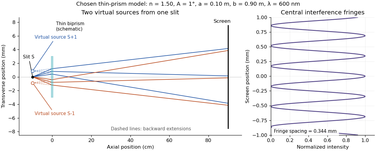
Two virtual sources and the interference fringes of a thin optical biprism
. Original paraxial model with the stated chosen parameters. Solid lines are selected physical rays; dashed lines extend the emergent rays backward to the virtual images. The prism is schematic, and axial and transverse scales differ. The right panel assumes equal coherent amplitudes and shows the central interference fringes, normalized to unit maximum. Details.A finite slit width, limited optical coherence, unequal beam intensities and misalignment can reduce fringe visibility. The Wollaston prism instead separates linear polarization components using birefringence; its two beams do not automatically interfere on an ordinary intensity screen because their polarizations are orthogonal.
Surface pressure integration for airfoil lift reconstructs the pressure contribution to lift by summing the local surface pressure loads with their directions. With pointing from a two-dimensional body into the fluid, the force per unit span from its closed contour isThe uniform reference pressure cancels on the closed contour. This is a vector line integral, not the sum of positive pressure magnitudes.[ref]
Aerodynamic Forces by NASA Glenn Research Center. Variation in Pressure and Definitions of Lift and Drag
For upper and lower surfaces that are graphs over , their pressure contribution perpendicular to the chord isVertical end closures have no chord-normal pressure contribution. The pressure force parallel to the chord, , still matters when resolving flow-relative lift. With flow direction in aft/chord-normal axes, . Equating with lift needs a suitable angle of attack approximation. Pressure integration also omits the viscous stress contribution.
Finite pressure tappings require numerical integration. A composite trapezoidal rule integrates the linearly interpolated samples exactly; it need not integrate the actual unsampled distribution exactly. For an original example, let and place taps at . A second invented profile agrees at every tap but has an additional on and zero addition elsewhere. Both reconstructions give , while the second true integral is .
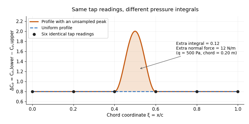
Two invented pressure-difference profiles agree at every tap but have different chord integrals. Equal readings alone do not bound an unsampled peak.
Details. At and , the two stipulated normal pressure forces are and , although the six samples are identical. This quadrature ambiguity of pressure-tap data is an instance of how finite samples do not certify quadrature accuracy. Additional geometric or regularity information is needed to bound the missed contribution.
A motivating experimental comparison uses a force balance independently of the pressure reconstruction. Robert M. Pinkerton's 54-orifice distribution measurements provide a historical example of resolving the shape of a pressure field.[ref]
Calculated and Measured Pressure Distributions over the Midspan Section of the NACA 4412 Airfoil by Robert M. Pinkerton. Abstract, apparatus and measured/theoretical distributions
A modern proposed test repeats both readings at controlled Reynolds number and angle of attack, checks tap coordinates and pressure-channel response, and refines sampling near sharp features. Agreement in a single integrated load does not prove agreement in the entire pressure distribution or pitching moment.A pressure-tap position error assigns a measured surface pressure to the wrong point on an airfoil. This differs from a pressure transducer's pressure-reading error: an accurate instrument can faithfully measure the pressure at a misplaced or incorrectly labeled hole. A steep spatial pressure gradient makes a small location error important.
Let be the nominal chord coordinate and let the actual pressure tapping lie at . For a differentiable pressure coefficient profile,If the derivative is bounded by throughout the interval between the two positions, the mean value theorem gives the rigorous bound . Knowing only an endpoint slope does not establish that bound across an unresolved peak.
In an original local example, take , a physical position error , and a profile locally linear with . Then and . At dynamic pressure , the corresponding pressure difference is . These are stipulated values illustrating sensitivity, not measurements of a particular airfoil.
For fixed quadrature weights and small errors in several tap positions, put . If is their position-error covariance matrix, the first-order variance contribution to a reconstructed coefficient isThis formula retains correlated position errors of pressure taps, including a shared coordinate-origin error. It holds the reconstruction weights and surface geometry fixed; uncertainty in those also needs accounting when geometry is inferred from the same coordinates.
Pressure-tap position calibration measures the actual hole coordinates and their reference origin, alongside pressure-channel calibration. Robert M. Pinkerton's distributed-pressure experiment used 54 orifices on an airfoil model to compare a measured distribution with potential flow predictions.[ref]
Calculated and Measured Pressure Distributions over the Midspan Section of the NACA 4412 Airfoil by Robert M. Pinkerton. Abstract, pressure-orifice distribution and theoretical comparison
Such a comparison tests both where a feature occurs and how large it is; pressure-only calibration cannot fix a displaced coordinate.Surface pressure, in fluid-mechanical loading, is the local pressure evaluated at a boundary such as an airfoil surface. It is a scalar field over position and time, with units of pascals. The field can vary strongly along the same body even when the surrounding free-stream conditions are fixed.
For a small surface patch with outward unit normal vector pointing from the solid into the fluid, the pressure contribution to the force isIt acts normally to the surface. Tangential viscous stress is a separate contribution. Experiments commonly compare the boundary value with a reference pressure using the pressure coefficientwhere is dynamic pressure. A coefficient is dimensionless; reconstructing the pressure difference requires the reference conditions.
For an original patch example, let , and . Then . On a patch, absolute pressure gives an inward force of ; relative to the reference pressure, the pressure-force contribution differs by outward. A negative coefficient therefore describes a reference-relative deficit, not a negative absolute pressure.
A primary wind tunnel experiment by Robert M. Pinkerton used 54 pressure orifices in a NACA4412 model and compared measured distributions at different angles of attack with potential flow predictions. Such pressure tapping observes local boundary pressures through small openings; the distribution is reconstructed from measurements at selected positions.[ref]
Calculated and Measured Pressure Distributions over the Midspan Section of the NACA 4412 Airfoil by Robert M. Pinkerton. NACA-TR-563, NTRS abstract: 54 orifices, tested incidence range and comparison with calculations
Spatial resolution of surface-pressure measurements limits what that reconstruction can establish between taps. Reference pressure, probe response and flow unsteadiness also affect the result. Surface pressure integration for airfoil lift uses the reconstructed field and surface directions to obtain an overall force; one pressure reading alone does not determine lift.
Unpremultiplication converts premultiplied alpha colour samples back to straight alpha by dividing out a nonzero alpha channel. If is the stored premultiplied colour triple, thenThe alpha value is retained. PNG's encoder guidance specifies this division when converting associated input samples to its unassociated representation, followed by scaling to the output sample range and rounding.[ref]
For an original exact-arithmetic example in Linear-light RGB, let and . The recovered colour is . Multiplying that triple by the retained alpha restores . Dividing the alpha itself would instead destroy the transparency information.
At , all exact premultiplied colour triples arising from finite equal zero. The original colour cannot be recovered from that result: many inputs mapped to the same stored value. PNG's conversion guidance chooses black for this case; that is a defined output convention, not recovered hidden colour.[ref]
Finite precision adds another limitation. Suppose , , and the premultiplied channels are rounded to eight-bit normalized codes. Their integer codes become , while the alpha code is one. Unpremultiplication then yields normalized straight colour , far from the original triple. For fixed exact alpha, a stored component error becomes after division. Near-zero alpha can therefore magnify rounding error even when the conversion formula is correct.
The Clavien-Dindo classification is an ordered severity classification for postoperative complications, based principally on the treatment needed to manage a deviation from the normal postoperative course. The 2004 proposal by Daniel Dindo, Nicolas Demartines and Pierre-Alain Clavien revised an earlier system and tested the revision using a 6,336-patient cohort and an international surgeon survey.[ref]
The main grades summarize different management consequences. Grade I permits only the limited measures specified in the original definition. Grade II includes additional pharmacological treatment and the specified categories of transfusion or nutritional support. Grade III requires surgical, endoscopic or radiological intervention; IIIa and IIIb distinguish whether general anaesthesia is used. Grade IV concerns a life-threatening complication requiring intermediate or intensive care, with subdivisions for single- and multiple-organ dysfunction. Grade V denotes death. The original table supplies the precise exceptions and qualifications.[ref]
The scale is ordered, not a ruler with equal intervals. Grade IV does not mean “twice as severe” as grade II. A numerical mean of grade labels consequently requires a justification beyond their ordering. Reporting the proportions in each category preserves information that a single average can hide.
Consider two illustrative groups of ten people. In each group, one person’s highest complication grade is III and the other nine have none. A highest-grade summary is identical. If the first affected person has one event and the second has three separate events, the summary still does not distinguish their total complication burden. Thus the unit of analysis, repeated-event rule and follow-up interval belong in the report. The original cohort analysis explicitly recorded the most severe complication when a patient had several.[ref]
Classification of Surgical Complications: A New Proposal With Evaluation in a Cohort of 6336 Patients and Results of a Survey by Daniel Dindo and others. Validation section, rule for multiple complications
The classification makes outcome descriptions more reproducible, but assigning a grade is distinct from establishing why an event occurred or which care strategy would have prevented it. It is most informative alongside clear case definitions and the wider evaluation of perioperative care.
Intrinsic positive end-expiratory pressure is the residual alveolar pressure above the externally imposed end-expiratory pressure, associated with incomplete lung emptying. In a communicating passive compartment,The manufacturer's technical account makes this distinction and explains why a fitted whole-breath estimate can differ from the pressure obtained during an end-expiratory hold.[ref]
Measurement of AutoPEEP and total PEEP by Hamilton Medical. Opening definition; Measuring AutoPEEP; Calculations
An original repeated-breath model isolates the timing mechanism. Let be excess volume above equilibrium with the outlet just before inspiration, and let each inspiration add tidal volume . During exhalation, assume a passive linear compartment with time constant . After expiratory time ,The steady excess volume satisfies , henceFor stipulated L, respiratory-system compliance L/cm HO, s and s, , L and intrinsic pressure is about 4.66 cm HO. Giving this same ideal compartment two seconds to empty yields about 0.063 L and 1.25 cm HO. These are consequences of a model, not patient-specific timing instructions.
A nonzero external baseline does not by itself imply incomplete emptying. Conversely, setting an external baseline to zero does not prove that alveolar pressure has returned to zero. Measurements require attention to communication between regions, leakage and active muscle pressure; a single airway value need not reveal every trapped regional pressure. The recurrence explains why resistance, compliance and available time matter together rather than assigning the phenomenon to one pressure setting alone.
An end-expiratory hold is an interruption of airflow at the end of exhalation during which airway pressure is observed while the respiratory system is occluded. In an appropriate passive, leak-free measurement it can assess total positive end-expiratory pressure, including intrinsic positive end-expiratory pressure. The set external pressure alone need not equal this measured total.[ref]
How to measure driving pressure by Hamilton Medical. End-expiratory hold and measurement conditions
The mechanical reason is easiest to see in one communicating compartment. With airway resistance , let relate airflow to the difference between alveolar pressure and measured airway pressure. Once flow vanishes and pressure has equilibrated through the communicating airway, this model gives . Zero flow removes the resistive pressure drop; it does not mean that either pressure is zero.
For stipulated pressures, an external setting of and an equilibrated total of differ by . If plateau airway pressure is , respiratory driving pressure is , whereas subtracting the external setting would give 18. These constructed values illustrate reference selection, not patient settings.
Occlusion changes the boundary condition rather than directly opening every lung region to the sensor. A compartment isolated by airway closure cannot be assumed to equilibrate with the measured opening. Active muscular effort, a leak or a pressure trace that has not settled also defeats the simple passive-compartment inference. The observed airway-pressure plateau and the inferred regional alveolar pressure must therefore remain distinct.
Unidirectional positioning repeatability describes the scatter of repeated returns to one commanded position when the final approach direction is held fixed. Specify the complete reset-and-return procedure so that each trial approaches under comparable conditions. PI distinguishes this directional scatter from its summaries that include reversal effects.[ref]
How to Consistently Verify the Performance of Nanopositioning Motion Control Equipment by Physik Instrumente. Sections3.1 and4.4, approach direction and unidirectional repeatability
For an original example, always approach from below. At a 2 mm target, suppose the position errors are ; at an 8 mm target they are . The means are and , respectively, while both sample standard deviations areThe same repeatability statistic accompanies quite different mean errors along the travel. A common shift of every reading at a target changes its mean but not its within-target spread.
For illustration, an explicitly declared specification taking the largest tested directional sample deviation would report for these two data sets. A specification using a full width or a multiple of that deviation would have a different numerical value. PI's own published convention states which directional spreads and target aggregation it uses; compare like definitions rather than only their units.[ref]
How to Consistently Verify the Performance of Nanopositioning Motion Control Equipment by Physik Instrumente. Section4.4, stated maximum/average unidirectional conventions
Observe final platform motion with an independent position readout, not just the motor's rotary encoder. Allow the chosen settling time and keep load and environment controlled. Consistently approaching from one side does not establish bidirectional positioning repeatability, and a small return scatter does not show that a small incremental command can be executed: that is the separate question of minimum incremental motion.
Bidirectional positioning repeatability concerns repeated arrivals at a commanded position using both approach directions. Retain the direction labels: the combined behavior can include both return-to-return scatter and a positioning reversal error. The manufacturer's method forms direction-specific means and spreads before reporting an axis-level summary over several targets.[ref]
How to Consistently Verify the Performance of Nanopositioning Motion Control Equipment by Physik Instrumente. Sections4.1–4.4, directional means and repeatability aggregation
For an original example, independently read the following errors at one target, in micrometres:The means are 0.2 and 1.2, and each direction has sample standard deviation . If a declared analysis pools all six observations, its sample variance decomposes exactly asHere the within-direction sum of squares is and the between-direction term is . Consequently,The larger pooled spread is mostly explained by approach direction. This is an original variance identity with a stated sample-standard-deviation convention, not a replacement definition for every manufacturer's repeatability tolerance.
A physical study repeatedly traverses the target from both sides and records final settled displacement with independent metrology. Report target positions, approach distances, order, load and environmental conditions. A directional mean difference may be almost invisible if only within-direction scatter is reported; pooling without direction labels hides its cause. Neither statistic alone establishes measurement accuracy, and one target does not characterize the full travel range.
A positioning reversal error compares the mean reached positions at one command when approached from opposite directions. Define for target , trial and approach direction . With denoting approach in the increasing-coordinate direction, use the signed target-specific quantityState this sign convention. PI's axis-level quantity called maximum positioning backlash instead takes the maximum absolute directional mean difference over the tested targets.[ref]
How to Consistently Verify the Performance of Nanopositioning Motion Control Equipment by Physik Instrumente. Section4.3, maximum absolute difference of directional means
For an original two-target example, measured mean errors at are from below and from above, giving . At , means of and give . ThusA small signed average can conceal substantial reversal effects that change sign along the travel.
Read final load position independently, for example with an interferometer, after an agreed settling time. The observed difference does not identify a unique physical cause: backlash, elastic relaxation or instrumental drift can contribute. For an original drift model , an unbalanced timing schedule givesAt and mean measurement times 50 s and 150 s, drift alone contributes . Alternate or balance the approach timing when testing that confounding effect. Unidirectional positioning repeatability measures within-direction scatter rather than this difference of means.
Digit reversal reverses a numeral's digit string in a specified radix and width. If has exactly displayed digits, allowing leading zeros, defineIt is an involution on the width- strings: reversing twice restores every digit to its original position.
In four-bit binary representation, reverses to , so the numbers three and twelve are paired at that width. With canonical decimal numerals, reverses to the displayed string , whose numerical value is . Reversing the canonical numeral then gives , so dropping width and leading zeros destroys the involution property.
The polynucleotide phosphorylase central channel is the passage through the ring-shaped protein trimer formed by polynucleotide phosphorylase. It helps organize RNA access to catalytic regions of the assembly. The channel is a property of the assembled enzyme, rather than a hollow tube inside one isolated polypeptide.[ref]
Different experiments supply different levels of evidence. The 2000 structure contained a phosphate analogue but no bound RNA and proposed a channel role in processivity. A 2021 cryo-electron microscopy study captured an RNA-containing state of a mycobacterial enzyme, including a terminal oligonucleotide in an active site and an adenine base in the central tunnel. That directly places substrate features in the assembly without resolving every segment of a complete chain.[ref]
Structure and mechanism of Mycobacterium smegmatis polynucleotide phosphorylase by Mihaela-Carmen Unciuleac and others. Abstract and Results, RNA-bound reconstructions; Figure4
A conceptual geometry test illustrates the importance of routing. Imagine an RNA with a flexible single-stranded tail followed by a bulky paired region. A channel admitting the tail need not admit that paired region. Entry, retention and bond cleavage can therefore impose different constraints on the observed reaction, even when the chemical active site is unchanged.
The structural observation should not be interpreted as a molecular movie. Mobility, unresolved density and transitions between catalytic states require biochemical or kinetic evidence alongside the static structure. In particular, a ring-shaped assembly alone does not prove unlimited processivity.
Pinned article: Introduction to the OurBigBook Project
Welcome to the OurBigBook Project! Our goal is to create the perfect publishing platform for STEM subjects, and get university-level students to write the best free STEM tutorials ever.
Everyone is welcome to create an account and play with the site: ourbigbook.com/go/register. We belive that students themselves can write amazing tutorials, but teachers are welcome too. You can write about anything you want, it doesn't have to be STEM or even educational. Silly test content is very welcome and you won't be penalized in any way. Just keep it legal!
Intro to OurBigBook
. Source. We have two killer features:
- topics: topics group articles by different users with the same title, e.g. here is the topic for the "Fundamental Theorem of Calculus" ourbigbook.com/go/topic/fundamental-theorem-of-calculusArticles of different users are sorted by upvote within each article page. This feature is a bit like:
- a Wikipedia where each user can have their own version of each article
- a Q&A website like Stack Overflow, where multiple people can give their views on a given topic, and the best ones are sorted by upvote. Except you don't need to wait for someone to ask first, and any topic goes, no matter how narrow or broad
This feature makes it possible for readers to find better explanations of any topic created by other writers. And it allows writers to create an explanation in a place that readers might actually find it.
Figure 1. Screenshot of the "Derivative" topic page. View it live at: ourbigbook.com/go/topic/derivativeVideo 2. OurBigBook Web topics demo. Source. - local editing: you can store all your personal knowledge base content locally in a plaintext markup format that can be edited locally and published either:This way you can be sure that even if OurBigBook.com were to go down one day (which we have no plans to do as it is quite cheap to host!), your content will still be perfectly readable as a static site.
- to OurBigBook.com to get awesome multi-user features like topics and likes
- as HTML files to a static website, which you can host yourself for free on many external providers like GitHub Pages, and remain in full control

Figure 2. You can publish local OurBigBook lightweight markup files to either OurBigBook.com or as a static website.
Figure 3. Visual Studio Code extension installation.
Figure 5. . You can also edit articles on the Web editor without installing anything locally. Video 3. Edit locally and publish demo. Source. This shows editing OurBigBook Markup and publishing it using the Visual Studio Code extension. 
- Infinitely deep tables of contents:




All our software is open source and hosted at: github.com/ourbigbook/ourbigbook
Further documentation can be found at: docs.ourbigbook.com
Feel free to reach our to us for any help or suggestions: docs.ourbigbook.com/#contact