
Markov chain Monte Carlo Created 2026-09-24 Updated 2026-11-05
Markov chain Monte Carlo estimates expectations under a target probability distribution by simulating a Markov chain that preserves . For an integrable observable , the assumptions of a Markov-chain law of large numbers justifyalmost surely. A Gibbs sampler preserves the target through full conditional distributions; a Metropolis–Hastings algorithm proposes a move and accepts or rejects it using a ratio of target and proposal densities. The unknown normalization constant cancels from that ratio, which makes unnormalized Bayesian posterior densities usable.
Successive states are generally dependent, so Monte Carlo precision depends on the observable's integrated autocorrelation time, rather than the raw iteration count alone. Burn-in can reduce initial-state effects but is not a proof of convergence. A correct stationary distribution also does not ensure rapid exploration: isolated modes or strong dependence can produce a long mixing time. Markov chain Monte Carlo convergence diagnostics investigate these limitations.
Bayes estimator Created 2026-09-24 Updated 2026-11-05
A Bayes estimator chooses an action minimizing posterior expected loss after observing data:The answer depends on the loss function: squared error gives the posterior mean, absolute error a posterior median, and discrete zero-one loss a posterior mode. For squared error, expanding proves the mean rule when the second moment is finite. Pointwise posterior minimization also minimizes integrated Bayes risk under the usual measurability and integrability conditions.
Bayesian posterior Created 2026-09-24 Updated 2026-10-14
The Bayesian posterior is the conditional probability distribution of an unknown statistical parameter after observing data. Suppose a continuous prior distribution has prior density relative to Lebesgue measure , and is the sampling probability mass function or probability density function of the observed data in the statistical model. Bayes' theorem givesThe Bayesian model evidence is the normalization constant making the posterior density integrate to one. The strict positive, finite condition is essential: a zero or infinite normalizer does not define this posterior distribution, even if the unnormalized expression can be written down. Other reference measures give the corresponding density formula; discrete parameter values replace the integral by a sum. The posterior propriety article gives examples where normalization fails.
With fixed, is a likelihood function of . Its normalization as a sampling distribution is over possible data, not over parameter values. In particular, a likelihood function is not a probability density function for and need not integrate to one over . The prior density supplies the probability weighting, and the Bayesian model evidence normalizes their product. This distinction prevents a tempting mistake: reversing the conditioning merely by exchanging the words “data” and “parameter”.
For eight heads among ten conditionally independent Bernoulli trials, take the observed data to be the heads count . Its binomial distribution likelihood function and the prior density giveUsing the Euler beta function , the Bayesian model evidence and normalized posterior density areThus the posterior distribution is . If the data are instead one particular ordered sequence with eight heads and two tails, its likelihood function omits the factor 45 and its Bayesian model evidence becomes . The factor cancels in Bayes' theorem, leaving the same posterior distribution; these two data descriptions have different sampling probabilities but identical information about here.
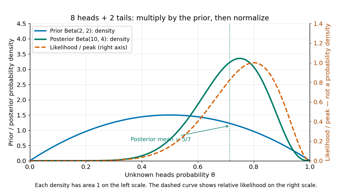
Beta(2,2) prior, peak-normalized Bernoulli likelihood, and Beta(10,4) posterior after eight heads and two tails
. Details. 
The prior density and posterior density use the left axis and each integrate to one. The dashed likelihood function uses the right axis and is divided by its maximum solely to compare its shape; it is not a parameter probability density function. The likelihood function peaks at , while the posterior mode is and the posterior mean is . Multiplying by the prior density shifts the preferred values toward one half while preserving a range of possibilities.
The resulting posterior variance is , compared with prior variance . In this example the update reduces uncertainty. The posterior predictive probability of heads on the next conditionally independent toss is , and the credible interval above reports a 95% range. These are summaries of the same posterior distribution, rather than competing estimates of one density peak.
Prior probability Created 2026-09-24 Updated 2026-10-14
Prior probability describes uncertainty before the current observations are incorporated. For a statistical parameter , a prior distribution assigns probabilities to its possible ranges, conditional on background information and a statistical model. A continuous prior density specifies these probabilities through integration:Here the probability density function is relative to Lebesgue measure ; a discrete prior distribution instead uses a probability mass function and sums. Density at one point is not the probability of that point. A nonnegative kernel with infinite total mass is an improper prior, whose use requires a separate check of posterior propriety.
For the coin model in Bayesian statistics, the beta distribution has prior density on . Its mean is and its variance is . It favors moderate heads probabilities without ruling out values near zero or one. For example,The prior curve in Bayesian posterior makes this preference visible; moment matching for a beta prior explains how to choose a beta distribution from a desired mean and variance.
A prior distribution lets earlier evidence or elicited knowledge contribute to statistical inference when the current sample size is limited. It also exposes assumptions that can be checked by prior elicitation and a prior predictive check. Before the same eight heads and two tails, a uniform prior would give posterior mean , compared with under : the observations do not uniquely determine a Bayesian posterior. Even a uniform prior makes a choice of parameter coordinates; its child article explains why changing coordinates can destroy uniformity.
Klein bottle group Created 2026-09-24 Updated 2026-10-03
Normal form theorem for an amalgamated free product Created 2026-09-24 Updated 2026-10-14
In , an alternating product of elements of and is nonidentity. More generally, choosing coset representatives gives a unique reduced normal form.
This is the amalgamated case of normal form for free groups and free product of groups.
HNN extension Created 2026-09-24 Updated 2026-10-14
Given isomorphic subgroups and an isomorphism , the HNN extension isIts stable letter records the loop edge in the associated graph of groups.
Bass-Serre tree Created 2026-09-24 Updated 2026-10-03
For , the Bass-Serre tree has vertices and edges , with joining to . Vertex degrees are the indices of the corresponding images of .
Epidemic invasion threshold Created 2026-09-24 Updated 2026-10-14
Fundamental theorem of linear programming Created 2026-09-24 Updated 2026-11-05
For a linear program in standard equality form , , a finite attained optimum has an optimal basic feasible solution. After deleting redundant equality rows, assume has full row rank. The nonnegative standard form is part of the statement: an arbitrary polyhedron containing lines can have an optimum and no extreme point.
Choose an optimal feasible vector with the fewest positive coordinates. If its positive-support columns are dependent, there is a nonzero vector supported there with . Both signs of a sufficiently small displacement remain feasible. Optimality forces , or one sign would improve the objective. Reverse if necessary so it has a negative coordinate, and increase until the first positive coordinate becomes zero. The objective is unchanged, contradicting minimal positive support. Thus those columns are independent and the solution is basic.
For contrast, minimizing the constant zero on the unrestricted real line has an optimum at every point, but no extreme points. Converting such a model to nonnegative standard form introduces a different polyhedron where the basis theorem applies. The theorem guarantees a place to find an optimum; it does not guarantee that every optimum is a vertex or that a particular pivot rule is fast.
Path reversal Created 2026-09-24 Updated 2026-09-24
Based homotopy Created 2026-09-24 Updated 2026-10-25
A based homotopy between based loops keeps both endpoints fixed at the base point throughout the deformation.
Constant-equation-of-state density scaling Created 2026-09-24 Updated 2026-10-05
Scale height of an isothermal atmosphere Created 2026-09-24 Updated 2026-10-20
This is the constant scale height of an isothermal atmosphere. The pressure and density decay length in an isothermal atmosphere is .
C-star algebra Created 2026-09-24 Updated 2026-11-05
A C-star algebra is a complex Banach algebra with an algebra involution satisfying the C-star identityThe algebra involution is conjugate-linear, reverses products and obeys . An identity need not be present.[ref]
Examples include complex matrices with the operator norm and conjugate transpose, bounded linear operators on a Hilbert space with the operator adjoint, and on a Hausdorff space that is a locally compact space with pointwise complex conjugation and the supremum norm. The identity ties the norm to the algebraic product and involution: it implies spectral radius norm equality for normal elements and makes an injective C-star homomorphism an isometry. This rigidity permits continuous functional calculus for normal C-star elements.
Banach subalgebra generated by one element Created 2026-09-24 Updated 2026-11-05
For in a complex unital Banach algebra , the closed unital subalgebra it generates is . Its character space is identified with by : polynomial density forces uniqueness, and spectrum equals character values in a commutative Banach algebra gives existence.
The ambient algebra matters. Spectrum of a polynomial-generated Banach subalgebra shows that is the full spectrum of in , including all bounded complementary components of . For example, in the coordinate has spectrum the unit circle, whereas is the boundary realization of the disk algebra and is the closed unit disk. Consequently it is the complement of , rather than necessarily that of , which is connected.
Character of an algebra Created 2026-09-24 Updated 2026-10-14
Algebra characters form the domain of the Gelfand representation; they are distinct from traces of group representations.
Spectrum of an element Created 2026-09-24 Updated 2026-10-14
Neumann series Created 2026-09-24 Updated 2026-10-20
If belongs to a unital Banach algebra and , thenAbsolute convergence and multiplication of partial sums prove the identity.
Unitization of an algebra Created 2026-09-24 Updated 2026-11-05
The unitization of a complex associative algebra is with productIts identity is , and identifies with a two-sided ideal. If is a Banach algebra, the norm makes a unital Banach algebra with the original norm on . The product formula directly proves submultiplicativity.[ref]
For a noncompact Hausdorff space that is a locally compact space, adjoining constant functions identifies the unitization of algebraically with , where is the one-point compactification. This does not identify the displayed sum norm with the supremum norm: those are equivalent norms, but the C-star unitization uses the latter. Unitization lets definitions such as the spectrum of an element apply to algebras that initially have no identity.
There are unlisted articles, also show them or only show them.