
Reflexive relation Created 2026-09-24 Updated 2026-10-14
Neyman-Pearson decision region Created 2026-09-24 Updated 2026-09-24
The Neyman-Pearson lemma says that an optimal region accepting has the likelihood-ratio formwith possible randomization on the boundary.
Stein's lemma (information theory) Created 2026-09-24 Updated 2026-10-14
For distinct probability distributions , the optimal error exponents in hypothesis testing give type-II error decay rate among tests whose type-I error stays below any fixed number in .
Dyadic rational Created 2026-09-24 Updated 2026-11-05
A dyadic rational is a rational number of the form with an integer and a nonnegative integer . Examples are , , zero and every integer. In lowest terms, its denominator is a power of two, so its magnitude has a finite binary expansion.
A positive dyadic rational also has a binary representation ending in infinitely many ones. Replacing the last nonzero binary digit by zero and filling all lower places with ones preserves the value, becauseFor example, . Zero has no second nonnegative expansion of this type. The same ambiguity applies to the magnitude of a negative dyadic rational, with its sign kept separately.
Hamming distance Created 2026-09-24 Updated 2026-10-03
The Hamming distance between two equal-length words is the number of coordinates in which they differ.
Nash equilibrium Created 2026-09-24 Updated 2026-10-14
A Nash equilibrium is a strategy profile in which every player's strategy is a best response to the others. For a finite game and mixed strategies, its precise condition isThe opponents' strategies are held fixed while testing each unilateral deviation. Equality is allowed: a player may have other equally good best responses. Because expected payoff is a linear function of the player's own mixture, it suffices to test every pure strategy. Equivalently, every choice in the support of a mixed strategy must attain the largest pure-choice expected payoff, and no unused choice may exceed it.
The two worked examples illustrate different uses of this condition. Matching pennies has no pure strategy Nash equilibrium, but its unique mixed strategy Nash equilibrium removes each player's vulnerability to predictable play. The asymmetric coordination example has three Nash equilibria, and its mixed one fails Pareto efficiency. A Nash equilibrium tests individual incentives, whereas Pareto efficiency compares feasible outcomes that may require several players to change together. In the prisoner's dilemma, for example, mutual defection is a Nash equilibrium even though mutual cooperation gives both players a larger payoff because .
Existence in a finite game is guaranteed by Nash's theorem. The theorem does not select one Nash equilibrium, promise Pareto efficiency, or assert convergence of a learning process. Nash's [ref] used the Kakutani fixed-point theorem; his [ref]
https://cs.uwaterloo.ca/~klarson/teaching/F04-886/papers/nash51.pdf. 1951 paper, section Existence of Equilibrium Points
gave a proof using the Brouwer fixed-point theorem. The connection to a fixed point captures the idea of choices that remain mutually optimal when considered together. Inertia of a bilinear form Created 2026-09-24 Updated 2026-11-05
The inertia of a real symmetric bilinear form is the triple giving the numbers of positive, negative, and zero squares in a diagonalization. Sylvester's law of inertia makes it independent of the chosen basis.
Nondegenerate bilinear form Created 2026-09-24 Updated 2026-10-14
A bilinear form is nondegenerate when its left radical and right radical are both zero: every nonzero vector can be detected by some pairing, whichever input slot it occupies. On a finite-dimensional vector space, either condition implies the other, and the following tests are equivalent:Here is the matrix of a bilinear form, and is the dual space. The linear map has matrix in the chosen basis and its dual basis, so its kernel is the right radical. The map has matrix . An invertible matrix has zero kernel on both sides, proving the finite-dimensional equivalence. In infinite dimensions, zero left radical and right radical imply these maps are injective, but do not generally make them surjective.[ref]
For the real symmetric bilinear form , the determinant is . Its isotropic vector has zero self-pairing but pairs to with , so it is detected. The alternating bilinear form with matrix has determinant and detects every nonzero vector even though all self-pairings vanish. Neither zero self-pairings nor the absence of positive definiteness implies degeneracy.
Nondegeneracy is useful because it turns a linear functional into a unique vector. For , the linear functional is ; solving for that representing vector amounts to solving an invertible system of linear equations. The analogous identification underlies bilinear orthogonal complements and the dual isomorphisms induced by a nondegenerate pairing.
Radical of a bilinear form Created 2026-09-24 Updated 2026-10-14
For a symmetric bilinear form or an alternating bilinear form, the radical is the linear subspaceThese vectors are invisible to all pairings, and the bilinear form is nondegenerate exactly when this linear subspace is . In coordinates, for both kinds of bilinear form, since or . Thus has radical of a bilinear form .
Passing to the quotient vector space removes precisely the invisible directions. The rule is well-defined because adding a vector in the radical of a bilinear form to either input changes no pairing, and the resulting bilinear form is nondegenerate. For , this quotient vector space retains just the direction and its form is ordinary multiplication.[ref]
https://www.math.ucla.edu/~rse/oldbook/Kniga.pdf. Elman, Karpenko and Merkurjev, The Algebraic and Geometric Theory of Quadratic Forms, §1: radical and nondegenerate quotient
For a general bilinear form, distinguish the left radical of a bilinear form from the right radical of a bilinear form; they can be different linear subspaces even though their dimensions agree in finite dimensions.
Degenerate bilinear form Created 2026-09-24 Updated 2026-10-14
A bilinear form is degenerate if some nonzero vector pairs to zero with every vector on at least one side. For a symmetric bilinear form or an alternating bilinear form, this says its radical of a bilinear form contains a nonzero vector. On a finite-dimensional vector space, it is equivalent to a singular matrix of a bilinear form, or .
For , . The nonzero vector is invisible to every pairing, and changing never changes . The quadratic form therefore has two parallel lines as its unit level set. This is a lost direction, a stronger condition than being an isotropic vector: with , but .
Coercive bilinear form Created 2026-09-24 Updated 2026-10-14
A real bilinear form on a normed vector space is coercive when there is one constant such thatThe lower bound uniformly controls every direction in the chosen norm. Unlike the upper bound defining a bounded bilinear form, it forces positive diagonal values at every nonzero vector. No symmetry is assumed. For complex Hilbert spaces, the usual analogue uses a sesquilinear form and ; it is not the same assertion for a complex bilinear form.
A concrete bounded and coercive example on , with the Euclidean norm, isIts quadratic form isThe best lower constant is , attained at . Nevertheless, and , so coercivity does not imply a symmetric bilinear form. The symmetric part of a matrix determines , while the skew-symmetric matrix part changes mixed pairings without changing . This is the symmetric and alternating parts of a bilinear form decomposition.[ref]
For the upper constant, direct multiplication gives . Its eigenvalues are , so the optimal upper constant, the spectral norm, is . The two constants answer different questions: how large a mixed pairing can be, and how small a self-pairing can be relative to squared norm.
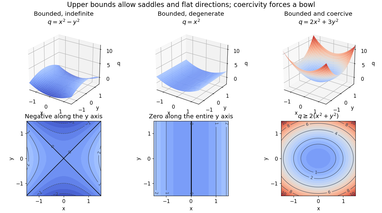
Bounded saddle and flat-direction quadratic forms contrasted with a uniformly coercive bowl
. Details. 
The plotted quadratic forms show the mechanism: descends in one direction, leaves one direction uncontrolled, and controls both. These are self-pairings; their level sets cannot reveal the skew-symmetric matrix part. Calling a quadratic energy here refers to this diagnostic quantity, not to a claim that a nonsymmetric equation comes from minimizing an energy functional.
On a real finite-dimensional vector space with any norm, strict positivity for every nonzero does imply coercivity. Indeed the quadratic form is continuous, and its positive minimum on the compact unit sphere supplies . If is also a symmetric bilinear form, this is positive definiteness. For general , it is the symmetric and alternating parts of a bilinear form decomposition that isolates the positive part. Switching between equivalent norms preserves coercivity, but usually changes its constant.
The infinite-dimensional vector space distinction is explicit on the real l2 sequence space:The Cauchy-Schwarz inequality gives boundedness with , and for every nonzero vector. But with , so no positive works. On the span of , the best lower constant is : each finite restriction is coercive, but the control disappears as grows. Strict positivity is therefore weaker than a uniform lower bound.
The practical payoff is a stability estimate for a weak formulation. Assume is a real Hilbert space, is both a bounded bilinear form and a coercive bilinear form, and the load is a bounded linear functional. The Lax-Milgram theorem gives a unique satisfying for all , including nonsymmetric .[ref]
Introduction to Finite Element Methods by Christian Clason. §2.2, Theorem 2.7, pp. 20–21, equation (2.9): hypotheses, unique solvability and load bound
The dual norm measures load size. Testing with gives the short energy estimateFor the bound holds directly; otherwise divide by . Subtracting the equations for two loads and using the same argument gives . Thus a positive lower constant limits the response to load errors. The upper bound and completeness of the Hilbert space enter the existence theorem; the estimate itself uses the lower bound and the load's dual norm.For the displayed matrix , take . Then for every means , not , with this ordering of the bilinear form. Since ,For , the exact response is and . For , it is , with norm . The actual maximal amplification is the operator norm : the coercivity estimate is valid but need not be sharp for a nonsymmetric bilinear form.
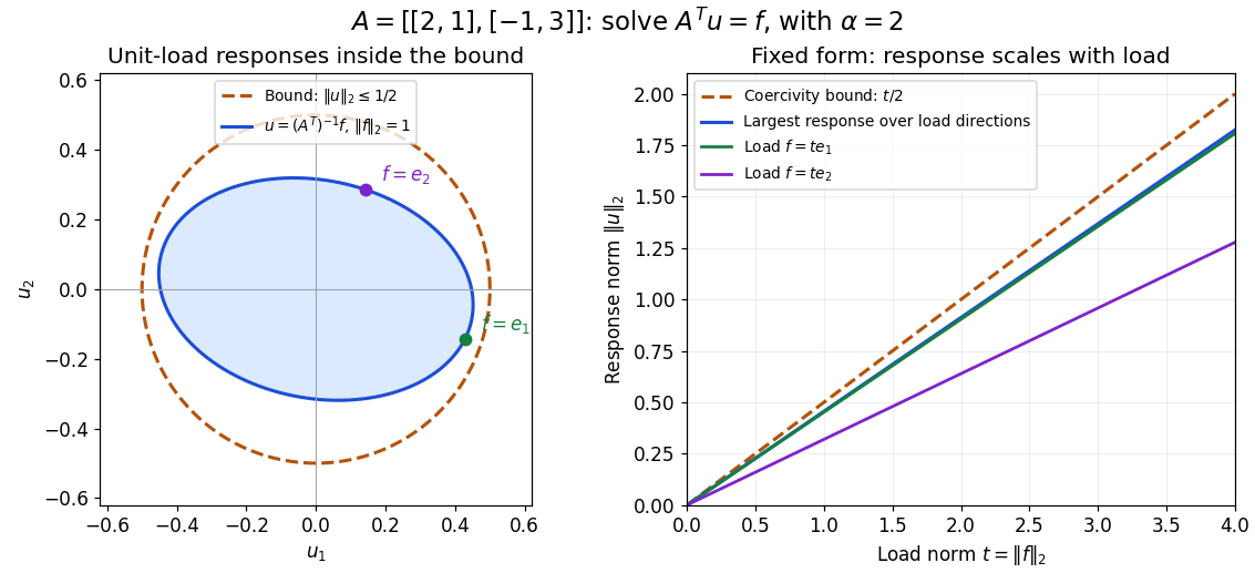
Solutions for unit loads lie inside the coercivity bound, and response grows at most linearly with load norm
. Details. 
Bounded bilinear form Created 2026-09-24 Updated 2026-10-14
A bilinear form on a real normed vector space is bounded when one constant satisfiesThis is an upper bound on the magnitude of every pairing. It says nothing about the sign of and does not require a symmetric bilinear form. The chosen norm is part of the hypothesis. Boundedness is equivalent to joint continuity, as shown by the boundedness criterion for a bilinear form.[ref]
For example, on with the Euclidean norm, the bilinear formsboth satisfy the upper bound with , by the Cauchy-Schwarz inequality. Yet their quadratic forms are and : the former takes negative values and the latter vanishes at the nonzero vector . Thus neither is a coercive bilinear form. The latter is also a degenerate bilinear form, whereas is nondegenerate. Boundedness controls size, not positivity or loss of directions.
Every bilinear form on a real or complex finite-dimensional vector space equipped with any norm is bounded. In coordinates, write using its matrix of a bilinear form. The Cauchy-Schwarz inequality gives , with the spectral norm; finite-dimensional equivalence of norms transfers this to the chosen norm. The conclusion concerns each fixed norm and fixed bilinear form: it does not supply a single constant for an arbitrary family of matrices or changing dimensions.
On an infinite-dimensional vector space, the upper bound is an additional condition. Equip the finitely supported sequences with the norm inherited from the l2 sequence space and setEach pairing is a finite sum, so this is a well-defined bilinear form. For the basis vector , however, and ; no finite works. It is even a coercive bilinear form with , since . Consequently coercivity alone does not imply boundedness on a normed vector space. This example uses , which is not a Hilbert space; it does not define this pairing on all of the l2 sequence space.
A bounded bilinear form defines a bounded linear operator by , where is the continuous dual space. Its operator norm is the smallest admissible :This converts an upper bound for pairings into an upper bound for a linear map taking an unknown vector to a linear functional.
Bifurcation diagram of the 2023 Cambridge quadratic-product system Created 2026-09-24 Updated 2026-09-24
The equilibria of , lie onfor every , and on for . They meet in a subcritical pitchfork bifurcation at ; the positive square-root branch meets the branch and exchanges stability in a transcritical bifurcation at .
Draining time of a uniform tank through a siphon Created 2026-09-24 Updated 2026-11-05
Consider a tank of constant cross-sectional area and a siphon of constant area . The tube outlet lies a vertical distance below the inlet, while the initial tank level is above the inlet. Treat the established draining stage as quasisteady incompressible flow, neglect losses and assume a filled siphon with both the free surface and outlet at atmospheric pressure. The model excludes the startup transient.
If the current level above the inlet is and the outlet speed is , mass conservation gives . The Bernoulli equation including the moving free-surface velocity givesIntegrating from to zero yieldsThis is the time for the surface to reach the inlet in the stated ideal model. Tube friction, trapped gas, loss of the continuous liquid column or appreciable unsteady inertia change the result.
Bernoulli equation over topography Created 2026-09-24 Updated 2026-11-05
Consider a steady incompressible flow with zero vorticity past a gently varying bottom , write the velocity potential as , where is the uniform background speed and . Take upward and let be the background pressure at . The Bernoulli equation isKeeping first-order terms and evaluating at the bottom givesThe first term is the hydrostatic pressure change due to elevation; the second comes from the perturbed kinetic energy per unit volume. The symbol denotes bottom height, while denotes the perturbation velocity potential.
The linearized no-penetration boundary condition is . Thus the bottom geometry first determines a perturbation flow, whose tangential velocity supplies the dynamic pressure correction. The approximation neglects both the squared perturbation velocity and products of the small height with perturbation derivatives.
Bernoulli function Created 2026-09-24 Updated 2026-11-05
A Bernoulli function collects the terms that become constant along streamlines under the conditions of the Bernoulli equation. For a barotropic inviscid flow with conservative body force , a useful specific-energy convention isHere is the barotropic enthalpy function. At constant density, up to a reference constant.
For steady flow, the Euler momentum equation gives : is constant along each streamline. It need not have the same value on distinct streamlines in a rotational flow. Stating the normalization matters because multiplying by a constant density produces a pressure-unit form, whereas the displayed function has energy-per-mass units. Comparing a pressure term directly with specific kinetic energy without that normalization gives an inconsistent balance.
CHSH inequality Created 2026-09-24 Updated 2026-10-18
For local outcomes , the Clauser–Horne–Shimony–Holt inequality isAn arbitrary no-signalling correlation can reach the algebraic maximum , while quantum correlations are bounded by .
For a short proof of the local bound, fix a deterministic local hidden-variable model assignment. The combination is . Exactly one bracket vanishes and the other is , so every assignment contributes . Averaging with a single setting-independent probability distribution preserves the interval . Mixtures also cover stochastic local hidden-variable theories. Rejecting a different sample at each setting would invalidate precisely that common-average step.
The quantum bound follows just as economically. For Hermitian operators with , the CHSH inequality operator obeys . Each commutator has operator norm at most two, giving . The Polarization CHSH count model attains this bound without allowing either station to control the distant marginal probability distribution.
Local hidden-variable theory Created 2026-09-24 Updated 2026-11-05
Evidence lower bound Created 2026-09-24 Updated 2026-11-05
For likelihood , prior density , evidence , and approximation density , the evidence lower bound isWhenever the terms are well-defined, substituting into the Kullback-Leibler divergence gives . Nonnegativity of the divergence proves the lower bound; equality holds when almost everywhere. Variational inference maximizes this objective over a tractable family, trading an exact posterior for an optimization problem.
Bayesian model averaging Created 2026-09-24 Updated 2026-09-24
Bayesian model averaging weights each model-specific posterior by that model's posterior probability.
There are unlisted articles, also show them or only show them.