
Power law Created 2026-09-24 Updated 2026-10-13
A power law is a relation , with fixed constants and . For positive , any real number is allowed. Its useful feature is a simple scaling rule:The same proportional change of input produces the same proportional change of output, independently of the starting value. The exponent controls that response; the coefficient fixes the magnitude.
For example, the area of a circle is . Doubling the radius multiplies its area by four, and tripling it multiplies the area by nine. The volume of a sphere is : the same changes multiply its volume by eight and twenty-seven. The distinction explains why similarly shaped objects do not preserve their ratio of surface area to volume when their size changes.
When the output is positive, a logarithm turns the power law into a straight-line relation. Using positive reference values and ,These ratios are dimensionless quantities, so the formula also applies to physical measurements with units. Plotting both ratios on a logarithmic scale gives a line of slope . Changing a unit changes the numerical coefficient, while the exponent stays the same. Positive describes increasing values; negative describes decreasing values; gives a constant. The zero coefficient is a degenerate case with no useful logarithmic slope.
Exact scaling is stronger than regular variation. The function has a doubling ratio tending to four, but its logarithmic correction keeps growing. The diagram contrasts it with the exact power law .
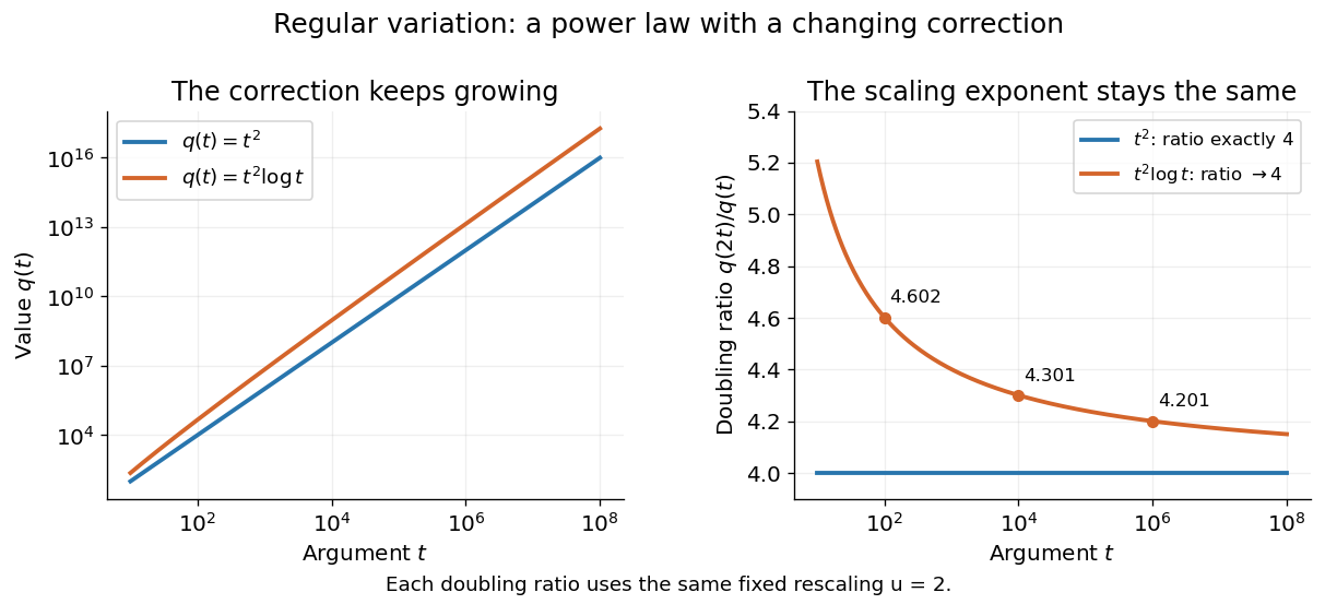
Exact quadratic scaling and a logarithmic correction have different finite doubling ratios, even though the correction leaves the limiting exponent unchanged
. Details. 
A power law for a probability density and a power law for a tail probability have different exponents. For a Pareto distribution with and lower endpoint one,The tail probability has exponent ; differentiating it and changing sign gives the probability density exponent . Confusing them changes the interpretation of a fitted exponent. The normalizing coefficient and lower endpoint also matter: a decreasing power law is not automatically a valid probability density over the entire positive real line.
The appearance of a line over a finite logarithmic range is evidence to investigate, rather than a proof of an exact power law or its mechanism. In their study of power-law distributions, Clauset, Shalizi and Newman combine maximum likelihood estimation, goodness-of-fit tests and comparisons with alternative models; their abstract explains why ordinary least-squares fitting can give misleading results for tail data. See Aaron Clauset, Cosma Rohilla Shalizi and M. E. J. Newman, Power-law distributions in empirical data, SIAM Review 51 (2009), 661–703. The scaling rule is mathematically exact when it defines a model; whether a dataset supports that model is a question of statistical inference.
Noncommutative algebra Created 2026-09-24 Updated 2026-11-05
Noncommutative algebra studies rings and algebras without assuming . Matrix algebras, group algebras, and Weyl algebras are central examples. The order of multiplication becomes part of the mathematical data.
For instance, a left ideal is closed under multiplication on the left, while a right ideal is closed under multiplication on the right; only a two-sided ideal supports a quotient ring. Likewise left and right modules can differ. Studying their categories through Morita equivalence often reveals similarities between rings that are not themselves isomorphic.
Commutative algebra Created 2026-09-24 Updated 2026-11-05
Commutative algebra studies commutative rings, ideals, modules, and the spectrum of a ring. Its basic question is which familiar rules of integer and polynomial arithmetic survive in a new setting. The distinction between units, zero divisors, and integral domains makes that question concrete.
Homogeneous polynomial Created 2026-09-24 Updated 2026-11-05
A nonzero polynomial is homogeneous of degree when every monomial with nonzero coefficient has total polynomial degree . Equivalently, the formal polynomial identityholds with an extra indeterminate . For example, is homogeneous of degree two, whereas mixes degrees. The zero polynomial is commonly included in every homogeneous component.
Over an infinite field, testing the scaling equation at all scalar values also detects homogeneity. Over a finite field, equality of polynomial functions is weaker than a formal polynomial identity: vanishes everywhere on despite mixing degrees. The monomial definition avoids that ambiguity. Homogeneity is what lets a zero set descend to projective space, since scaling a nonzero coordinate representative does not change whether the polynomial vanishes.
Group theory Created 2026-09-24 Updated 2026-10-14
A group records reversible operations that can be combined consistently. Group theory studies their subgroups, group homomorphisms, group actions, and quotient groups. A symmetry group makes the abstraction visible: transformations may change individual points while preserving a specified object or its structure. An orbit of a group action records which positions can be exchanged, while a stabilizer subgroup records which operations leave a selected feature fixed.
Fundamental theorem of algebra Created 2026-09-24 Updated 2026-11-05
Every nonconstant complex polynomial has a complex root and therefore factors completely into linear factors over .
Unit in a ring Created 2026-09-24 Updated 2026-11-05
A unit in a unital ring is an element with a two-sided multiplicative inverse :The ring is part of the condition. In the only units are and , whereas every nonzero rational number is a unit in . Modulo six, is a unit because , while is a nonunit.
In a nonzero ring, zero is never a unit, since . Every unit has multiplicative cancellation, but a cancellable element need not be a unit: can be cancelled in the integers, yet its reciprocal is not an integer. The units form the unit group of the ring.
Unique factorization domain Created 2026-09-24 Updated 2026-11-05
A unique factorization domain is an integral domain in which every nonzero nonunit factors into finitely many irreducible elements, uniquely up to reordering and multiplying individual factors by units. Existence and uniqueness are both required. The integers and the polynomial ring over a field are examples.
In a unique factorization domain, every irreducible element is a prime element. Comparing prime factorizations therefore justifies cancellation of common factors and the usual exponent rules for a greatest common divisor. The integral domain fails uniqueness, as gives inequivalent factorizations into irreducible elements.
Transcendental number Created 2026-09-24 Updated 2026-11-05
A transcendental number is a complex number that is not an algebraic number. No nonzero polynomial with coefficients in the integers vanishes at it. Familiar examples are and ; proving their transcendence requires substantially more than proving their irrationality.
There are only countably many integer-coefficient polynomials, and each nonzero one has finitely many roots. Consequently the algebraic numbers are countable, while the real numbers are uncountable; transcendental real numbers therefore exist in abundance. This counting proof establishes existence without identifying a particular example. Every real transcendental number is an irrational number, but shows that the converse fails.
Surjective function Created 2026-09-24 Updated 2026-11-05
A function is surjective when every element of its codomain occurs as a value: for each there is an with . Equivalently, its image is all of .
For example, is surjective as a function , but not as a function , since negative values are missed. A surjective function may identify different inputs. Together with injectivity, surjectivity gives a bijection and hence an inverse function.
Star-shaped set Created 2026-09-24 Updated 2026-11-05
A subset of a real vector space is a star-shaped set if some point sees every point of along a segment lying in : for all and . Every convex set is star-shaped about each of its points; a star-shaped set need only have one such point.
For example, the union of the horizontal and vertical line segments through the origin is star-shaped about the origin but is not convex. In a topological vector space, the map contracts a star-shaped set to . This makes it contractible, a useful bridge from elementary geometry to homotopy theory.
Smith normal form Created 2026-09-24 Updated 2026-11-05
For every matrix over a principal ideal domain, there are invertible matrices such thatThe nonzero diagonal entries are unique up to multiplication by units. Over the integers, and are unimodular and the may be chosen positive; their products are the greatest common divisors of the -rowed minors.
Root of unity Created 2026-09-24 Updated 2026-11-05
RSA cryptosystem Created 2026-09-24 Updated 2026-11-05
In the two-prime RSA cryptosystem, choose distinct odd prime numbers , set , and choose an integer coprime to . A private exponent satisfies . The public key is ; the private key permits the inverse modular exponentiation. For a message representative ,Correctness holds even when is not coprime to : modulo each prime the zero case is immediate, while the nonzero case follows from Fermat's little theorem; the Chinese remainder theorem recombines the two congruences.
For example, , , and give ; encrypts to and decrypts back to . These tiny parameters only illustrate the arithmetic. The raw deterministic exponentiation is textbook RSA; practical encryption uses an encoding scheme rather than encrypting an unencoded message directly.[ref]
Polynomial interpolation error Created 2026-09-24 Updated 2026-11-05
Let be the interpolation polynomial through at distinct interpolation nodes . If has continuous derivatives on an interval containing the nodes and a point , thenfor some in that interval. At a node the error is zero. Away from the nodes, subtract a suitable multiple of the product so the resulting function vanishes at the nodes and at ; repeated Rolle's theorem gives the formula.[ref]
For linear interpolation, this yields if . The product explains why the placement of interpolation nodes matters. The intermediate point depends on and must not be treated as a constant when differentiating an error formula.
Pigeonhole principle Created 2026-09-24 Updated 2026-10-18
Place objects into boxes, assigning each object to exactly one box. Here is a nonnegative integer and is a positive integer. The pigeonhole principle says that if , some box contains at least two objects. Equivalently, a function from an -element finite set to an -element finite set cannot be an injective function when . The boxes may stand for categories rather than physical containers. [ref]
https://ocw.mit.edu/courses/6-042j-mathematics-for-computer-science-spring-2015/mit6_042js15_textbook.pdf#page=581. Lehman, Leighton and Meyer, Mathematics for Computer Science, section 14.8, rule 14.8.1
For thirteen objects and twelve boxes, a box containing at least two is unavoidable. Thinking of thirteen people and their birth months gives the same conclusion: at least two share a birth month. Twelve people could occupy the twelve months one apiece, so thirteen is the smallest number that forces a shared month. The generalized pigeonhole principle quantifies how many objects must share a box when there are still more objects.
The useful surprise is that the pigeonhole principle proves existence without needing to locate the objects involved. Choosing a good assignment rule is often the creative step: equal labels can mean equal remainders, nearby points, or repeated states of an algorithm. Once the rule is chosen, a short count can force a relationship among a much larger collection of objects. The pigeonhole principle itself does not name the crowded box. When the objects and their assignments are explicitly available, a simple algorithm finds one: scan the objects, keep the first object seen in each box, and stop when a later object enters an occupied box. At most scanned objects are needed when .
A geometric example. Any five points in a square of side one contain two whose Euclidean distance is at most . Give each point Cartesian coordinates . Divide both ranges into the intervals and , making four cells. Thus belongs to the left half and to the right half; belongs to the lower half and to the upper half. This convention assigns every boundary point to exactly one cell.
The pigeonhole principle puts two of the five points in the same cell. Their differences in Cartesian coordinates have magnitude at most , so the Pythagorean theorem gives their Euclidean distance the boundFor the plotted points , , , and , the first two occupy the lower-left cell and have Euclidean distance . These Cartesian coordinates exhibit the forced pair; the argument applies to every placement of five points.
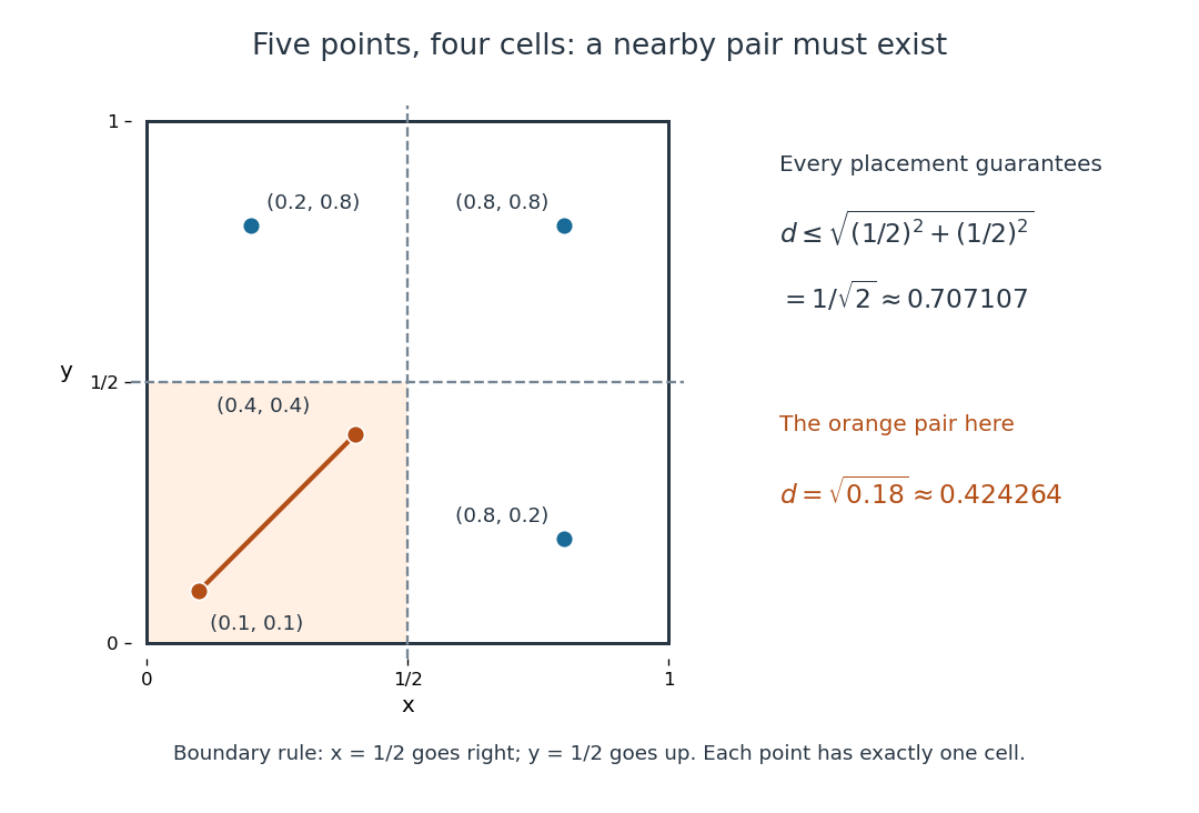
The pigeonhole principle places two of five points in one of four cells of a square, bounding their Euclidean distance by
. Details. 
An arithmetic example. Assign eight integers to their seven residue classes modulo the integer modulus . The pigeonhole principle gives two with the same residue class, so is an integer divisor of their difference. In , for example, and satisfy the integer congruence , and . Likewise, assigning fractional parts to short intervals gives the Dirichlet approximation theorem; its existing article explains the approximation bound.
Noetherian ring Created 2026-09-24 Updated 2026-11-05
A commutative ring is Noetherian if each of its ideals has a finite generating set. Equivalently, every increasing chain of ideals eventually stops growing. For the equivalence, the union of an increasing chain is an ideal; its finitely many generators already lie in one member. Conversely, repeatedly adjoining an element outside the generated ideal would produce a nonterminating chain.
The integers are a Noetherian ring, since each ideal is principal. The Hilbert basis theorem then shows that is Noetherian. The infinitely generated polynomial ring is not: never stabilizes. The condition ensures that finitely many equations suffice to describe each ideal, even when its elements form an infinite set.[ref]
Nilpotent polynomial Created 2026-09-24 Updated 2026-11-05
A polynomial over a commutative ring is a nilpotent element if for some positive integer . This happens exactly when all its coefficients are nilpotent elements of . For example, is a nilpotent polynomial in , since its square is zero.
If the finitely many coefficients satisfy , every product of more than coefficients contains a vanishing factor, proving one direction. Conversely, reduce modulo any prime ideal: the resulting polynomial ring is an integral domain, so a nilpotent image must be zero. Each coefficient therefore belongs to every prime ideal, hence to the nilradical. In particular a polynomial ring over a reduced ring is reduced.
Minimal number of generators Created 2026-09-24 Updated 2026-11-05
The minimal number of generators of a group, module, ideal, or algebraic structure is the smallest size of a generating set for the specified operations. The type of structure matters: generating a ring as an ideal, as an algebra, and as an additive group are different questions.
For a finitely generated module over a local ring with residue field , Nakayama's lemma gives . Every generating set maps to a spanning set, giving the lower bound; lifts of a basis generate by Nakayama's lemma, giving equality. For example, the ideal in needs two generators, since its quotient by has basis given by the classes of .
Mathematical induction Created 2026-09-24 Updated 2026-10-14
A mathematical induction proof establishes a property for every integer by proving its induction base case and its inductive step. If a counterexample existed, the well-ordering principle would give a least one; its predecessor and the inductive implication exclude it. The starting case excludes a counterexample at .
The useful idea is to cover infinitely many cases with two finite pieces of reasoning. The induction base case starts the chain, and the inductive step shows that success at an arbitrary stage propagates to the next. It is especially natural when a construction adds one item at a time: another row of a diagram, another input processed by an algorithm, or another term of a sequence. The loop invariant method is the same propagation idea applied to successive stages of a computation.
For the triangular number , the proposed formula is . At , both sides are one. Assuming the formula for a fixed positive integer , add the next row:This is the desired formula at , proving the inductive step. For example, and ; these numerical cases illustrate the general step rather than replace it.
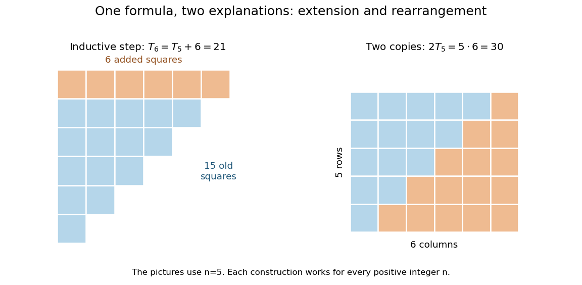
Adding the next row gives the induction step; rearranging two triangular arrays gives the same formula geometrically
. Details. 
The second picture explains where the formula comes from: two copies of the triangular arrangement tile an by rectangle. Thus . The mathematical induction argument certifies how the formula continues, while the rearrangement makes its factors visible. Neither picture is restricted to the five rows drawn: both constructions are specified for every positive integer .
There are unlisted articles, also show them or only show them.